Describe & Vizualize

Date: September 10, 2025

A fuzzy monster in a beret and scarf, critiquing their own column graph on a canvas in front of them while other assistant monsters (also in berets) carry over boxes full of elements that can be used to customize a graph (like themes and geometric shapes). In the background is a wall with framed data visualizations. Stylized text reads “ggplot2: build a data masterpiece.” Learn more about ggplot2.

# File management
library(here)
# for dplyr, ggplot2
library(tidyverse)
#Loading data
library(rio)
# for descriptives
library(psych)

#Remove Scientific Notation 
options(scipen=999)

Starting Up

Let’s first start by opening our Project

Then, create a new Notebook/Markdown Document that we will use for today

Setup the libraries and bring in the data

We will use the TIPI data from the last lecture that has already been scored

#import data - Your path may be different
tipi <- import(here("files", "data", "final_tipi.csv")) %>% 
  # from the janitor package
  janitor::clean_names()

Summarizing Data

So far we have been calculating various descriptive statistics (somewhat painstakingly) using an assortment of different functions. So what if we have a dataset with a bunch of variables we want descriptive statistics for? Surely we don’t want to calculate descriptives for each variable by hand…

Fortunately for us, there is a function called describe() from the {psych} package, which we can use to quickly summarize a whole set of variables in a dataset.

Be sure to first install the package prior to putting it into your library code chunk. Reminder: anytime you add a library, be sure you actually run the code line library(psych). Otherwise, you will have a hard time trying to use the next functions.

Let’s use it with our dataset!

describe()

This function automatically calculates all of the descriptives we reviewed above (and more!). Use the describe() function from the psych package on the entire dataset.

Notes: If you load a library at the beginning, you can directly call any function from it. Instead, you can call a function by library_name::function_name without loading the entire library.

psych::describe(tipi)

                    vars  n    mean       sd median trimmed    mad    min
id                     1 99 1058.12    31.05 1059.0 1057.93  38.55 1006.0
progress               2 99  100.00     0.00  100.0  100.00   0.00  100.0
duration_in_seconds    3 99 7197.29 34904.64 1461.0 1527.88 486.29  623.0
consent                4 99    1.00     0.00    1.0    1.00   0.00    1.0
genderid               5 99    4.46     0.82    4.0    4.47   1.48    1.0
genderid_7_text*       6 99    1.03     0.22    1.0    1.00   0.00    1.0
sex                    7 99    1.51     0.50    2.0    1.51   0.00    1.0
age                    8 99   19.78     1.84   20.0   19.53   1.48   17.0
year_school            9 99    2.18     1.22    2.0    2.04   1.48    1.0
q85                   10 99    1.64     1.32    1.0    1.32   0.00    1.0
q85_6_text*           11 99    1.03     0.22    1.0    1.00   0.00    1.0
tipi_1                12 99    3.99     1.90    4.0    3.99   2.97    1.0
tipi_2                13 99    4.15     1.53    4.0    4.23   1.48    1.0
tipi_3                14 99    5.38     1.26    6.0    5.51   1.48    1.0
tipi_4                15 99    4.29     1.69    5.0    4.31   1.48    1.0
tipi_5                16 99    5.38     1.28    6.0    5.52   1.48    1.0
tipi_6                17 99    4.76     1.64    5.0    4.84   1.48    1.0
tipi_7                18 99    5.45     1.24    6.0    5.57   1.48    2.0
tipi_8                19 99    3.17     1.70    3.0    3.09   1.48    1.0
tipi_9                20 99    5.01     1.35    5.0    5.05   1.48    2.0
tipi_10               21 99    3.10     1.48    3.0    3.04   1.48    1.0
sleep_quality         22 99    2.56     1.15    2.0    2.46   1.48    1.0
hours_of_sleep        23 99    6.51     1.04    7.0    6.63   0.00    1.0
tipi_2r               24 99    3.85     1.53    4.0    3.77   1.48    1.0
tipi_4r               25 99    3.71     1.69    3.0    3.69   1.48    1.0
tipi_6r               26 99    3.24     1.64    3.0    3.16   1.48    1.0
tipi_8r               27 99    4.83     1.70    5.0    4.91   1.48    1.0
tipi_10r              28 99    4.90     1.48    5.0    4.96   1.48    1.0
extra                 29 99    3.62     1.60    3.5    3.56   2.22    1.0
agree                 30 99    4.65     1.08    4.5    4.63   0.74    2.0
consc                 31 99    5.11     1.22    5.5    5.15   1.48    2.0
emo                   32 99    4.36     1.29    4.5    4.37   1.48    1.5
open                  33 99    5.14     1.04    5.0    5.19   0.74    2.5
                       max    range  skew kurtosis      se
id                    1112    106.0  0.03    -1.21    3.12
progress               100      0.0   NaN      NaN    0.00
duration_in_seconds 252521 251898.0  6.57    42.24 3508.05
consent                  1      0.0   NaN      NaN    0.00
genderid                 7      6.0 -0.81     5.57    0.08
genderid_7_text*         3      2.0  7.70    61.15    0.02
sex                      2      1.0 -0.02    -2.02    0.05
age                     31     14.0  2.67    12.52    0.19
year_school              5      4.0  0.73    -0.44    0.12
q85                      7      6.0  2.18     4.14    0.13
q85_6_text*              3      2.0  7.70    61.15    0.02
tipi_1                   7      6.0  0.01    -1.34    0.19
tipi_2                   7      6.0 -0.46    -0.58    0.15
tipi_3                   7      6.0 -0.86     0.58    0.13
tipi_4                   7      6.0 -0.17    -0.95    0.17
tipi_5                   7      6.0 -0.94     0.86    0.13
tipi_6                   7      6.0 -0.46    -0.86    0.17
tipi_7                   7      5.0 -0.65    -0.08    0.12
tipi_8                   7      6.0  0.37    -1.12    0.17
tipi_9                   7      5.0 -0.29    -0.81    0.14
tipi_10                  7      6.0  0.35    -0.71    0.15
sleep_quality            5      4.0  0.87     0.14    0.12
hours_of_sleep           8      7.0 -2.01     5.99    0.10
tipi_2r                  7      6.0  0.46    -0.58    0.15
tipi_4r                  7      6.0  0.17    -0.95    0.17
tipi_6r                  7      6.0  0.46    -0.86    0.17
tipi_8r                  7      6.0 -0.37    -1.12    0.17
tipi_10r                 7      6.0 -0.35    -0.71    0.15
extra                    7      6.0  0.18    -0.98    0.16
agree                    7      5.0  0.11     0.04    0.11
consc                    7      5.0 -0.32    -0.70    0.12
emo                      7      5.5 -0.10    -0.54    0.13
open                     7      4.5 -0.48     0.13    0.10

# or if you have already loaded the library

describe(tipi)

                    vars  n    mean       sd median trimmed    mad    min
id                     1 99 1058.12    31.05 1059.0 1057.93  38.55 1006.0
progress               2 99  100.00     0.00  100.0  100.00   0.00  100.0
duration_in_seconds    3 99 7197.29 34904.64 1461.0 1527.88 486.29  623.0
consent                4 99    1.00     0.00    1.0    1.00   0.00    1.0
genderid               5 99    4.46     0.82    4.0    4.47   1.48    1.0
genderid_7_text*       6 99    1.03     0.22    1.0    1.00   0.00    1.0
sex                    7 99    1.51     0.50    2.0    1.51   0.00    1.0
age                    8 99   19.78     1.84   20.0   19.53   1.48   17.0
year_school            9 99    2.18     1.22    2.0    2.04   1.48    1.0
q85                   10 99    1.64     1.32    1.0    1.32   0.00    1.0
q85_6_text*           11 99    1.03     0.22    1.0    1.00   0.00    1.0
tipi_1                12 99    3.99     1.90    4.0    3.99   2.97    1.0
tipi_2                13 99    4.15     1.53    4.0    4.23   1.48    1.0
tipi_3                14 99    5.38     1.26    6.0    5.51   1.48    1.0
tipi_4                15 99    4.29     1.69    5.0    4.31   1.48    1.0
tipi_5                16 99    5.38     1.28    6.0    5.52   1.48    1.0
tipi_6                17 99    4.76     1.64    5.0    4.84   1.48    1.0
tipi_7                18 99    5.45     1.24    6.0    5.57   1.48    2.0
tipi_8                19 99    3.17     1.70    3.0    3.09   1.48    1.0
tipi_9                20 99    5.01     1.35    5.0    5.05   1.48    2.0
tipi_10               21 99    3.10     1.48    3.0    3.04   1.48    1.0
sleep_quality         22 99    2.56     1.15    2.0    2.46   1.48    1.0
hours_of_sleep        23 99    6.51     1.04    7.0    6.63   0.00    1.0
tipi_2r               24 99    3.85     1.53    4.0    3.77   1.48    1.0
tipi_4r               25 99    3.71     1.69    3.0    3.69   1.48    1.0
tipi_6r               26 99    3.24     1.64    3.0    3.16   1.48    1.0
tipi_8r               27 99    4.83     1.70    5.0    4.91   1.48    1.0
tipi_10r              28 99    4.90     1.48    5.0    4.96   1.48    1.0
extra                 29 99    3.62     1.60    3.5    3.56   2.22    1.0
agree                 30 99    4.65     1.08    4.5    4.63   0.74    2.0
consc                 31 99    5.11     1.22    5.5    5.15   1.48    2.0
emo                   32 99    4.36     1.29    4.5    4.37   1.48    1.5
open                  33 99    5.14     1.04    5.0    5.19   0.74    2.5
                       max    range  skew kurtosis      se
id                    1112    106.0  0.03    -1.21    3.12
progress               100      0.0   NaN      NaN    0.00
duration_in_seconds 252521 251898.0  6.57    42.24 3508.05
consent                  1      0.0   NaN      NaN    0.00
genderid                 7      6.0 -0.81     5.57    0.08
genderid_7_text*         3      2.0  7.70    61.15    0.02
sex                      2      1.0 -0.02    -2.02    0.05
age                     31     14.0  2.67    12.52    0.19
year_school              5      4.0  0.73    -0.44    0.12
q85                      7      6.0  2.18     4.14    0.13
q85_6_text*              3      2.0  7.70    61.15    0.02
tipi_1                   7      6.0  0.01    -1.34    0.19
tipi_2                   7      6.0 -0.46    -0.58    0.15
tipi_3                   7      6.0 -0.86     0.58    0.13
tipi_4                   7      6.0 -0.17    -0.95    0.17
tipi_5                   7      6.0 -0.94     0.86    0.13
tipi_6                   7      6.0 -0.46    -0.86    0.17
tipi_7                   7      5.0 -0.65    -0.08    0.12
tipi_8                   7      6.0  0.37    -1.12    0.17
tipi_9                   7      5.0 -0.29    -0.81    0.14
tipi_10                  7      6.0  0.35    -0.71    0.15
sleep_quality            5      4.0  0.87     0.14    0.12
hours_of_sleep           8      7.0 -2.01     5.99    0.10
tipi_2r                  7      6.0  0.46    -0.58    0.15
tipi_4r                  7      6.0  0.17    -0.95    0.17
tipi_6r                  7      6.0  0.46    -0.86    0.17
tipi_8r                  7      6.0 -0.37    -1.12    0.17
tipi_10r                 7      6.0 -0.35    -0.71    0.15
extra                    7      6.0  0.18    -0.98    0.16
agree                    7      5.0  0.11     0.04    0.11
consc                    7      5.0 -0.32    -0.70    0.12
emo                      7      5.5 -0.10    -0.54    0.13
open                     7      4.5 -0.48     0.13    0.10

NOTE: Some variables are not numeric and are categorical variables of type character. By default, the describe() function forces non-numeric variables to be numeric and attempts to calculate descriptives for them. These variables are marked with an asterisk (*). In this case, it doesn’t make sense to calculate descriptive statistics for these variables, so we get a warning message and a bunch of NaN’s and NA’s for these variables.

A better approach would be to remove non-numeric variables before you attempt to run numerical calculations on your dataset.

Make it Pretty

Using sjPlot (https://strengejacke.github.io/sjPlot/index.html) we can make things a little more publishable! You can use select() to also keep particular variables (maybe you don’t care about the skew)

tipi %>% 
  psych::describe() %>% 
  sjPlot::tab_df()

vars	n	mean	sd	median	trimmed	mad	min	max	range	skew	kurtosis	se
1	99	1058.12	31.05	1059.00	1057.93	38.55	1006.00	1112	106.00	0.03	-1.21	3.12
2	99	100.00	0.00	100.00	100.00	0.00	100.00	100	0.00	NaN	NaN	0.00
3	99	7197.29	34904.64	1461.00	1527.88	486.29	623.00	252521	251898.00	6.57	42.24	3508.05
4	99	1.00	0.00	1.00	1.00	0.00	1.00	1	0.00	NaN	NaN	0.00
5	99	4.46	0.82	4.00	4.47	1.48	1.00	7	6.00	-0.81	5.57	0.08
6	99	1.03	0.22	1.00	1.00	0.00	1.00	3	2.00	7.70	61.15	0.02
7	99	1.51	0.50	2.00	1.51	0.00	1.00	2	1.00	-0.02	-2.02	0.05
8	99	19.78	1.84	20.00	19.53	1.48	17.00	31	14.00	2.67	12.52	0.19
9	99	2.18	1.22	2.00	2.04	1.48	1.00	5	4.00	0.73	-0.44	0.12
10	99	1.64	1.32	1.00	1.32	0.00	1.00	7	6.00	2.18	4.14	0.13
11	99	1.03	0.22	1.00	1.00	0.00	1.00	3	2.00	7.70	61.15	0.02
12	99	3.99	1.90	4.00	3.99	2.97	1.00	7	6.00	0.01	-1.34	0.19
13	99	4.15	1.53	4.00	4.23	1.48	1.00	7	6.00	-0.46	-0.58	0.15
14	99	5.38	1.26	6.00	5.51	1.48	1.00	7	6.00	-0.86	0.58	0.13
15	99	4.29	1.69	5.00	4.31	1.48	1.00	7	6.00	-0.17	-0.95	0.17
16	99	5.38	1.28	6.00	5.52	1.48	1.00	7	6.00	-0.94	0.86	0.13
17	99	4.76	1.64	5.00	4.84	1.48	1.00	7	6.00	-0.46	-0.86	0.17
18	99	5.45	1.24	6.00	5.57	1.48	2.00	7	5.00	-0.65	-0.08	0.12
19	99	3.17	1.70	3.00	3.09	1.48	1.00	7	6.00	0.37	-1.12	0.17
20	99	5.01	1.35	5.00	5.05	1.48	2.00	7	5.00	-0.29	-0.81	0.14
21	99	3.10	1.48	3.00	3.04	1.48	1.00	7	6.00	0.35	-0.71	0.15
22	99	2.56	1.15	2.00	2.46	1.48	1.00	5	4.00	0.87	0.14	0.12
23	99	6.51	1.04	7.00	6.63	0.00	1.00	8	7.00	-2.01	5.99	0.10
24	99	3.85	1.53	4.00	3.77	1.48	1.00	7	6.00	0.46	-0.58	0.15
25	99	3.71	1.69	3.00	3.69	1.48	1.00	7	6.00	0.17	-0.95	0.17
26	99	3.24	1.64	3.00	3.16	1.48	1.00	7	6.00	0.46	-0.86	0.17
27	99	4.83	1.70	5.00	4.91	1.48	1.00	7	6.00	-0.37	-1.12	0.17
28	99	4.90	1.48	5.00	4.96	1.48	1.00	7	6.00	-0.35	-0.71	0.15
29	99	3.62	1.60	3.50	3.56	2.22	1.00	7	6.00	0.18	-0.98	0.16
30	99	4.65	1.08	4.50	4.63	0.74	2.00	7	5.00	0.11	0.04	0.11
31	99	5.11	1.22	5.50	5.15	1.48	2.00	7	5.00	-0.32	-0.70	0.12
32	99	4.36	1.29	4.50	4.37	1.48	1.50	7	5.50	-0.10	-0.54	0.13
33	99	5.14	1.04	5.00	5.19	0.74	2.50	7	4.50	-0.48	0.13	0.10

`ggplot2`

`ggplot2` from the `tidyverse`

Since we have already installed and loaded the library, we don’t have to do anything else at this point!

ggplot2 follows the “grammar of graphics”

Theoretical framework for creating data visualizations
Breaks the process down into separate components:

Data

Aesthetics (aes)

Geometric Objects (geoms)

Faceting

Themes

Grammar of Graphics

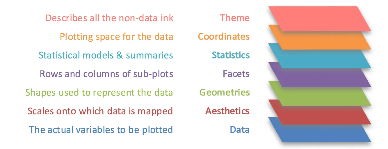
`ggplot2` cheatsheet

`ggplot2` syntax

There is a basic structure to create a plot within ggplot2, and consists of at least these three things:

A Data Set
Coordinate System
Geoms - visual marks to represent the data points

In R it looks like this:

ggplot(data = <DATA>) + 
  <GEOM_FUNCTION>(mapping = aes(<MAPPINGS>))

#or how I like to do it
<DATA> %>% 
  ggplot(aes(<MAPPINGS>)) + 
  <GEOM_FUNCTION>()

`ggplot2` syntax

Let’s start with a basic figure with our TIPI data

First we will define the data that we are using and the variables we are visualizing

#the dataset is called penguins

tipi %>% 
  #including the variables we want to visualize
  ggplot(aes(x = emo, 
             y = extra))

What happens?

We forgot to tell it what to do with the data!

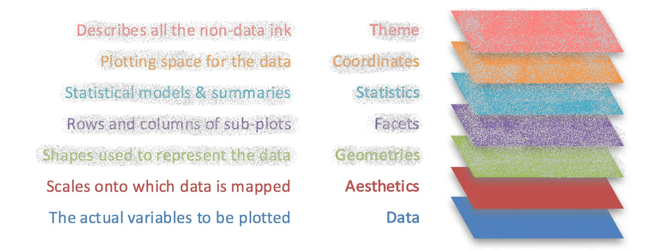
Need to add the appropriate geom to have it plot points for each observation

tipi %>% 
  ggplot(aes(x = emo, 
             y = extra)) + 
  geom_point()

Note: the geom_point() layer will “inherit” what is in the aes() in the previous layer

Adding in Color

Maybe we would like to have each of the points colored by their respective sex

This information will be added to the aes() within the geom_point() layer

tipi %>% 
  ggplot(aes(x = emo, 
             y = extra)) + 
  geom_point(aes(color=sex))

Including a fit line

Why don’t we put in a line that represents the relationship between these variables?

We will want to add another layer/geom

tipi %>% 
  ggplot(aes(x = emo, 
             y = extra)) + 
  geom_point(aes(color=sex)) + 
  geom_smooth()

That looks a little wonky…why is that? Did you get a note in the console?

Including a fit line

The geom_smooth() defaults to using a loess line to fit to the data

In order to update that, we need to change some of the defaults for that layer and specify that we want a “linear model” or lm function to the data

tipi %>% 
  ggplot(aes(x = emo, 
             y = extra)) + 
  geom_point(aes(color=sex)) + 
  geom_smooth(method = 'lm')

Did that look a little better?

Individual fit lines

It might make more sense to have individual lines for each of the species instead of something that is across all

tipi %>% 
  ggplot(aes(x = emo, 
             y = extra, 
             color = sex)) + 
  geom_point(aes(color=sex)) + 
  geom_smooth(method = 'lm')

What did we move around from the last set of code?

What was the error you got?

Data Types

It looks like R is looking at our binary variable as a continuous number

We want to be able to tell our code that these are categories/factors

If we want to change or compute a new variable, what do we use?

tipi <- tipi %>% 
  mutate(sex = as.factor(sex))

Let’s try that again:

tipi %>% 
  ggplot(aes(x = emo, 
             y = extra, 
             color = sex)) + 
  geom_point(aes(color=sex)) + 
  geom_smooth(method = 'lm')

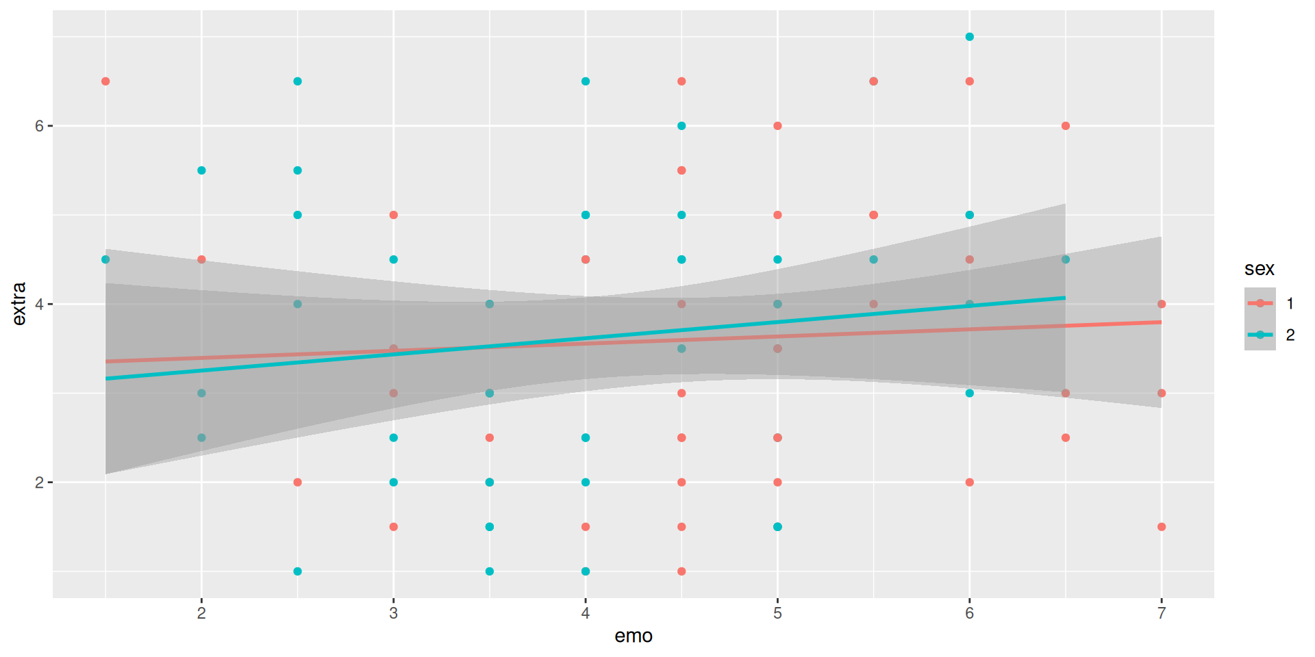
Updating Labels/Title

It will default to including the variable names as the x and y labels, but that isn’t something that makes sense. Also would be good to have a title!

We add on another layer called labs() for our labels (link)

tipi %>% 
  ggplot(aes(x = emo, 
             y = extra, 
             color = sex)) + 
  geom_point(aes(color=sex)) + 
  geom_smooth(method = 'lm') + 
  labs(
    title = "TIPI Data",
    subtitle = "Extraversion by Emotional Stability", 
    x = "motional Stability", 
    y = "Extraversion", 
    color = "Sex at Birth"
  )

Other Graphs

Take another look at the ggplot cheatsheet

What else is a useful chart?

Bar Charts

tipi %>% 
  ggplot(aes(x = duration_in_seconds)) + 
  geom_bar()

tipi %>% 
  ggplot(aes(x = age)) + 
  geom_bar(aes(fill = sex), 
                 alpha = 0.5, 
                 position = "identity")

Describe & Vizualize

Starting Up

Summarizing Data

describe()

Make it Pretty

ggplot2

ggplot2 from the tidyverse

Grammar of Graphics

ggplot2 cheatsheet

ggplot2 syntax

ggplot2 syntax

Adding in Color

Including a fit line

Including a fit line

Individual fit lines

Data Types

Let’s try that again:

Updating Labels/Title

Other Graphs

Bar Charts

`ggplot2`

`ggplot2` from the `tidyverse`

`ggplot2` cheatsheet

`ggplot2` syntax

`ggplot2` syntax