dplyr: Wrangling
Date: September 10, 2025
Starting Up
Let’s first start by opening our Project
Then, create a new Markdown Document that we will use for this activity
Setup the libraries and bring in the data
- We will use the TIPI data (Download from here)
Naming Conventions
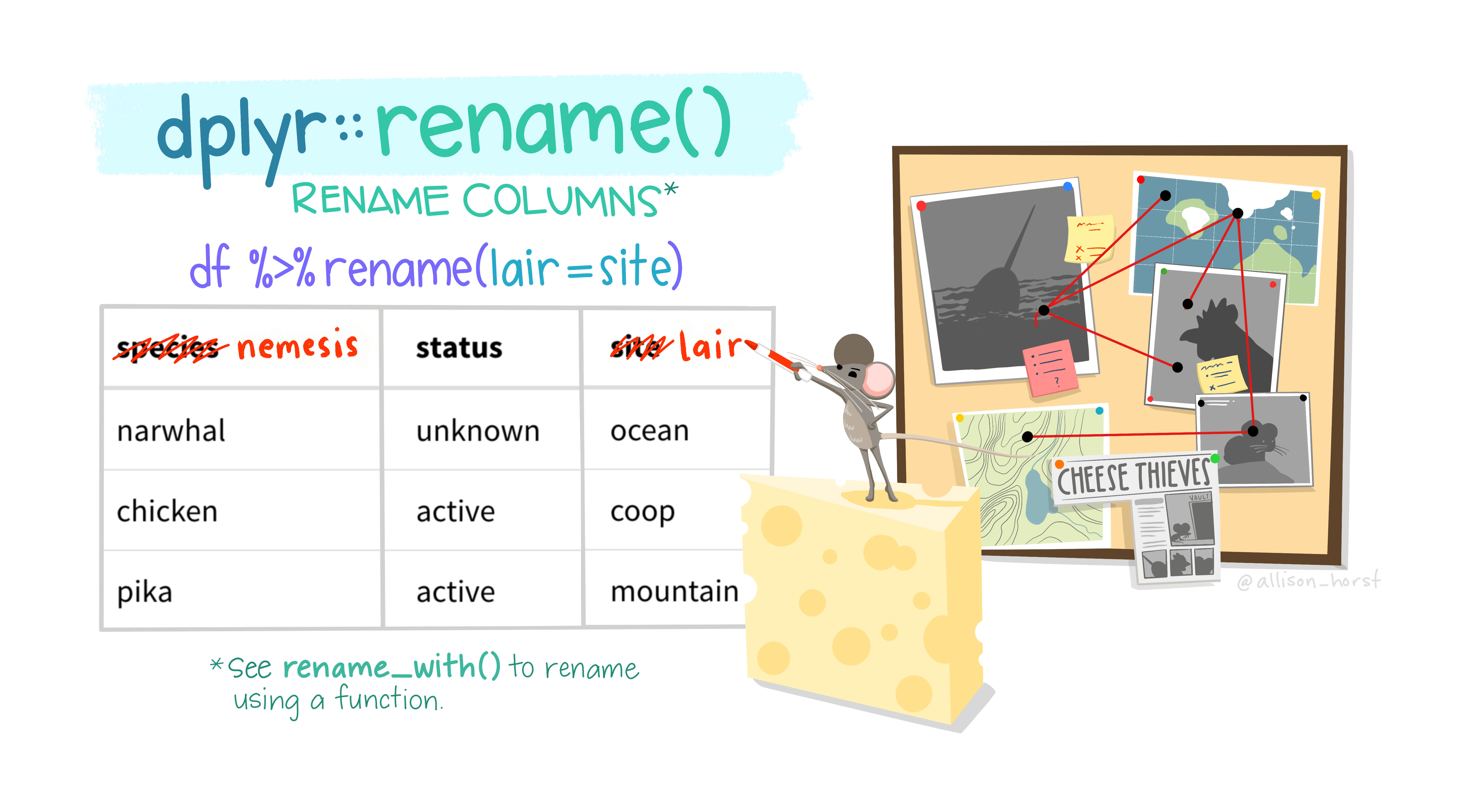
We could use the rename() function, but that take a lot of work. It can be helpful if you want to change it to something specific, but we may just want to make these names a little cleaner.
Introducing janitor https://sfirke.github.io/janitor/index.html
This function automatically puts column names into snake-case
#same code as before
tipi <- import(here("files", "data", "TIPI_Data.csv")) %>%
  # from the janitor package
  janitor::clean_names()
names(tipi)
[1] "id" "progress" "duration_in_seconds"
[4] "consent" "genderid" "genderid_7_text"
[7] "sex" "age" "year_school"
[10] "q85" "q85_6_text" "tipi_1"
[13] "tipi_2" "tipi_3" "tipi_4"
[16] "tipi_5" "tipi_6" "tipi_7"
[19] "tipi_8" "tipi_9" "tipi_10"
[22] "sleep_quality" "hours_of_sleep" select()
.png)
Using select()
You used this in lab, so you are all experts. Let’s review by looking at the cheatsheet for dplyr.
The dplyr package makes data wrangling and transformation much easier. select() allows you to…well…select the columns that you want to keep.
Create a dataset that only includes: id, progress, duration, sex, age, TIPI items and the sleep items
Using select()
filter()
.png)
Extract Rows
The ‘filter()’ function is used to subset observations based on their values.
The result of filtering is a data frame with the same number of columns as before but fewer rows.
The first argument is data and subsequent arguments are logical expressions that tell you which observations to retain in the data frame.
Note: You are stating which types of rows you want to keep. If a variable can answer TRUE to your condition, then it will stay in the data.
# A tibble: 38 × 14
   name     height  mass hair_color skin_color eye_color birth_year sex   gender
   <chr>     <int> <dbl> <chr>      <chr>      <chr>          <dbl> <chr> <chr>
 1 Darth V…    202   136 none       white      yellow          41.9 male  mascu…
 2 IG-88       200   140 none       metal      red             15   none  mascu…
 3 Bossk       190   113 none       green      red             53   male  mascu…
 4 Lobot       175    79 none       light      blue            37   male  mascu…
 5 Ackbar      180    83 none       brown mot… orange          41   male  mascu…
 6 Nien Nu…    160    68 none       grey       black           NA   male  mascu…
 7 Nute Gu…    191    90 none       mottled g… red             NA   male  mascu…
 8 Jar Jar…    196    66 none       orange     orange          52   male  mascu…
 9 Roos Ta…    224    82 none       grey       orange          NA   male  mascu…
10 Rugor N…    206    NA none       green      orange          NA   male  mascu…
# ℹ 28 more rows
# ℹ 5 more variables: homeworld <chr>, species <chr>, films <list>,
#   vehicles <list>, starships <list>
Filter Observations
We can now generate a subset of observations based on a particular value
There may be some data checks that you perform when wrangling data. One that I would suggest is to look at the overall completion percentages and the amount of time that it took for participants to complete the questionnaire.
This is exactly what filter() is set to do.
mutate()
.png)
Compute new variable
We often need to make a sum/mean score for a variable of interest, or transform it in some way.
The mutate() function is most commonly used to add new columns to your data frame that are functions of existing columns.
mutate() requires data as its first argument, followed by a set of expressions defining new columns.
- Note: New variables are automatically added at the end of the data frame (scroll to the right to see them)
For example, we have the Ten Item Personality Inventory
Take a look at the scoring of the TIPI and compute the necessary variables for all subscales
Reverse Coding
There are some items in questionnaire data that are rated in the opposite direction from the other items. These need to be “reverse coded” or “reverse scored”
The TIPI documention highlights certain variables that need this done
We can take the max value, add 1, then subtract the Item
coded_tipi_data <- clean_tipi_data %>%
  mutate(tipi_2r = 8 - tipi_2,
         tipi_4r = 8 - tipi_4,
         tipi_6r = 8 - tipi_6,
         tipi_8r = 8 - tipi_8,
         tipi_10r = 8 - tipi_10)

coded_tipi_data %>% select(tipi_2, tipi_2r, tipi_4, tipi_4r) %>% head()
tipi_2 tipi_2r tipi_4 tipi_4r
1 3 5 3 5
2 5 3 5 3
3 3 5 5 3
4 2 6 7 1
5 5 3 5 3
6 6 2 2 6Reverse Coding 2.0
With R, if there is something that is tedious, then that probably means that someone has made a library for it to make it easier.
Here comes reverse() from datawizard
datawizard::reverse()
We can try out this function with our TIPI data to see if we get something similar to before.
# renaming it something different in case we want to compare
wizard_tipi_data <- clean_tipi_data %>%
  datawizard::reverse(
    select = c("tipi_2", "tipi_4", "tipi_6", "tipi_8", "tipi_10"),
    append = "r"
  )

wizard_tipi_data %>% select(tipi_2, tipi_2r, tipi_4, tipi_4r) %>% head()
tipi_2 tipi_2r tipi_4 tipi_4r
1 3 5 3 5
2 5 3 5 3
3 3 5 5 3
4 2 6 7 1
5 5 3 5 3
6 6 2 2 6Sum Scores
And finally, we can use mutate() to create total scores (or really any type of computation)
For the TIPI data, we need to compute each of the 5 pieces of the Big Five (Extraversion, Agreeableness, Conscientiousness, Emotional Stability and Openness to Experience)
Exporting Data
export()
Now that we have a scored dataset, we will want to save that.
You can do this by re-running all of your steps above, or by exporting your dataset.
Note
Be careful when exporting and knitting docs. Each time you knit, it will run the export code. After I export, I usually will comment out that line of code.
