Unit 5 - Descriptives (pt. 2)
PSYC 640 - Fall 2024
Reminders
Journal Entries
Lab 1 - Now due 10/6
Last Class
- Focused on basic descriptives
mean()median()describe()
Today…
Explore correlations and comparing means.
Import cleaned up file
Last class we created a new .csv file named named_Sleep_Data. We will continue to use that! Let’s make sure to import that data.
Relationships between variables
Association - Correlation
Examine the relationship between two continuous variables
Similar to the mean and standard deviation, but it is between two variables
Typically displayed as a scatterplot

Association - Covariance
Before we talk about correlation, we need to take a look at covariance
\[ cov_{xy} = \frac{\sum(x-\bar{x})(y-\bar{y})}{N-1} \]
Covariance can be thought of as the “average cross product” between two variables
It captures the raw/unstandardized relationship between two variables
Covariance matrix is the basis for many statistical analyses
Covariance to Correlation
The Pearson correlation coefficient \(r\) addresses this by standardizing the covariance
It is done in the same way that we would create a \(z-score\)…by dividing by the standard deviation
\[ r_{xy} = \frac{Cov(x,y)}{sd_x sd_y} \]
Correlations
Tells us: How much 2 variables are linearly related
Range: -1 to +1
Most common and basic effect size measure
Is used to build the regression model
Interpreting Correlations (5.7.5)
| Correlation | Strength | Direction |
|---|---|---|
| -1.0 to -0.9 | Very Strong | Negative |
| -0.9 to -0.7 | Strong | Negative |
| -0.7 to -0.4 | Moderate | Negative |
| -0.4 to -0.2 | Weak | Negative |
| -0.2 to 0 | Negligible | Negative |
| 0 to 0.2 | Negligible | Positive |
| 0.2 to 0.4 | Weak | Positive |
| 0.4 to 0.7 | Moderate | Positive |
| 0.7 to 0.9 | Strong | Positive |
| 0.9 to 1.0 | Very Strong | Positive |
Pearson Correlations in R
Calculating Correlation in R
Now how do we get a correlation value in R?
That will give us the correlation, but we also want to know how to get our p-value
Correlation Test
To get the test of a single pair of variables, we will use the cor.test() function:
Using real data - Epworth Sleepiness Scale
So far we have been looking at single variables, but we often care about the relationships between multiple variables in a dataset
| ESS1m1 | ESS2m1 | ESS3m1 | ESS4m1 | ESS5m1 | ESS6m1 | ESS7m1 | ESS8m1 | |
|---|---|---|---|---|---|---|---|---|
| ESS1m1 | 1 | NA | NA | NA | NA | NA | NA | NA |
| ESS2m1 | NA | 1 | NA | NA | NA | NA | NA | NA |
| ESS3m1 | NA | NA | 1 | NA | NA | NA | NA | NA |
| ESS4m1 | NA | NA | NA | 1 | NA | NA | NA | NA |
| ESS5m1 | NA | NA | NA | NA | 1 | NA | NA | NA |
| ESS6m1 | NA | NA | NA | NA | NA | 1 | NA | NA |
| ESS7m1 | NA | NA | NA | NA | NA | NA | 1 | NA |
| ESS8m1 | NA | NA | NA | NA | NA | NA | NA | 1 |
Missing Values - na.rm = TRUE?
Handling Missing - Correlation
Listwise Deletion (complete cases)
- Removes participants completely if they are missing a value being compared
- Smaller Sample Sizes
- Doesn’t bias correlation estimate
Pairwise Deletion
- Removes participants for that single pair, but leaves information in when there are complete information
- Larger Sample Sizes
- Could bias estimates if there is a systematic reason things are missing
| ESS1m1 | ESS2m1 | ESS3m1 | ESS4m1 | ESS5m1 | ESS6m1 | ESS7m1 | ESS8m1 | |
|---|---|---|---|---|---|---|---|---|
| ESS1m1 | 1.0000000 | 0.3303236 | 0.2784836 | 0.1455593 | 0.2295289 | 0.1422071 | 0.2206383 | 0.0984444 |
| ESS2m1 | 0.3303236 | 1.0000000 | 0.1976108 | 0.1387409 | 0.2190331 | 0.1748049 | 0.2134999 | 0.1010883 |
| ESS3m1 | 0.2784836 | 0.1976108 | 1.0000000 | 0.2920448 | 0.1948408 | 0.2888370 | 0.2778982 | 0.2178073 |
| ESS4m1 | 0.1455593 | 0.1387409 | 0.2920448 | 1.0000000 | 0.2579808 | 0.0897873 | 0.2589136 | 0.2409171 |
| ESS5m1 | 0.2295289 | 0.2190331 | 0.1948408 | 0.2579808 | 1.0000000 | 0.0704590 | 0.2821851 | 0.0629151 |
| ESS6m1 | 0.1422071 | 0.1748049 | 0.2888370 | 0.0897873 | 0.0704590 | 1.0000000 | 0.2833070 | 0.3493524 |
| ESS7m1 | 0.2206383 | 0.2134999 | 0.2778982 | 0.2589136 | 0.2821851 | 0.2833070 | 1.0000000 | 0.2356524 |
| ESS8m1 | 0.0984444 | 0.1010883 | 0.2178073 | 0.2409171 | 0.0629151 | 0.3493524 | 0.2356524 | 1.0000000 |
Spearman’s Rank Correaltion
Spearman’s Rank Correlation
We need to be able to capture this different (ordinal) “relationship”
- If student 1 works more hours than student 2, then we can guarantee that student 1 will get a better grade
Instead of using the amount given by the variables (“hours studied”), we rank the variables based on least (rank = 1) to most (rank = 10)
Then we correlate the rankings with one another
Foundations of Statistics
Who were those white dudes that started this?
Statistics and Eugenics
The concept of the correlation is primarily attributed to Sir Frances Galton
- He was also the founder of the concept of eugenics
The correlation coefficient was developed by his student, Karl Pearson, and adapted into the ANOVA framework by Sir Ronald Fisher
- Both were prominent advocates for the eugenics movement
What do we do with this info?
Never use the correlation or the later techniques developed on it? Of course not.
Acknowledge this history? Certainly.
Understand how the perspectives of Galton, Fisher, Pearson and others shaped our practices? We must! – these are not set in stone, nor are they necessarily the best way to move forward.
Be aware of the assumptions
Statistics are often thought of as being absent of bias…they are just numbers
Statistical significance was a way to avoid talking about nuance or degree.
“Correlation does not imply causation” was a refutation of work demonstrating associations between environment and poverty.
Need to be particularly mindful of our goals as scientists and how they can influence the way we interpret the findings
Fancy Tables
Correlation Tables
Before we used the cor() function to create a correlation matrix of our variables
But what is missing?
| ESS1m1 | ESS2m1 | ESS3m1 | ESS4m1 | ESS5m1 | ESS6m1 | ESS7m1 | ESS8m1 | |
|---|---|---|---|---|---|---|---|---|
| ESS1m1 | 1.0000000 | 0.3303236 | 0.2784836 | 0.1455593 | 0.2295289 | 0.1422071 | 0.2206383 | 0.0984444 |
| ESS2m1 | 0.3303236 | 1.0000000 | 0.1976108 | 0.1387409 | 0.2190331 | 0.1748049 | 0.2134999 | 0.1010883 |
| ESS3m1 | 0.2784836 | 0.1976108 | 1.0000000 | 0.2920448 | 0.1948408 | 0.2888370 | 0.2778982 | 0.2178073 |
| ESS4m1 | 0.1455593 | 0.1387409 | 0.2920448 | 1.0000000 | 0.2579808 | 0.0897873 | 0.2589136 | 0.2409171 |
| ESS5m1 | 0.2295289 | 0.2190331 | 0.1948408 | 0.2579808 | 1.0000000 | 0.0704590 | 0.2821851 | 0.0629151 |
| ESS6m1 | 0.1422071 | 0.1748049 | 0.2888370 | 0.0897873 | 0.0704590 | 1.0000000 | 0.2833070 | 0.3493524 |
| ESS7m1 | 0.2206383 | 0.2134999 | 0.2778982 | 0.2589136 | 0.2821851 | 0.2833070 | 1.0000000 | 0.2356524 |
| ESS8m1 | 0.0984444 | 0.1010883 | 0.2178073 | 0.2409171 | 0.0629151 | 0.3493524 | 0.2356524 | 1.0000000 |
Correlation Tables - sjPlot
sleep_data %>%
  select(ESS1m1:ESS8m1) %>%
  cor(use = "complete") %>%
tab_corr(na.deletion = "listwise", triangle = "lower")| ESS1m1 | ESS2m1 | ESS3m1 | ESS4m1 | ESS5m1 | ESS6m1 | ESS7m1 | ESS8m1 | |
| ESS1m1 | ||||||||
| ESS2m1 | 0.330 | |||||||
| ESS3m1 | 0.278 | 0.198 | ||||||
| ESS4m1 | 0.146 | 0.139 | 0.292 | |||||
| ESS5m1 | 0.230 | 0.219 | 0.195 | 0.258 | ||||
| ESS6m1 | 0.142 | 0.175 | 0.289 | 0.090 | 0.070 | |||
| ESS7m1 | 0.221 | 0.213 | 0.278 | 0.259 | 0.282 | 0.283 | ||
| ESS8m1 | 0.098 | 0.101 | 0.218 | 0.241 | 0.063 | 0.349 | 0.236 | |
| Computed correlation used pearson-method with listwise-deletion. | ||||||||
Correlation Tables - sjPlot
So many different cusomizations for this type of plot
Can add titles, indicate what missingness and method
Saves you a TON of time when putting it into a manuscript
Writing up a Correlation
Template: r(degress of freedom) = the r statistic, p = p value.
Imagine we have conducted a study of 40 students that looked at whether IQ scores and GPA are correlated. We might report the results like this:
IQ and GPA were found to be moderately positively correlated, r(38) = .34, p = .032.
Other example:
Among the students of Hogwarts University, the number of hours playing Fortnite per week and midterm exam results were negatively correlated, r(78) = -.45, p < .001.
And another:
Table 1 reports descriptive statistics and correlations among variables of interest. Knowledge of Weird Al Songs was positively correlated with perceptions of humor for Dr. Haraden (r(49) = .79, p <.001), such that the more Weird Al songs a student knew, the more they thought Dr. Haraden was funny.
Visualizing Data
Visualizing Data
It is always important to visualize our data! Even after getting the correlations and other descriptives
Let’s look at some data:
Code
data1 <- import("https://raw.githubusercontent.com/dharaden/dharaden.github.io/main/data/data1.csv") %>%
  mutate(dataset = "data1")

data2 <- import("https://raw.githubusercontent.com/dharaden/dharaden.github.io/main/data/data2.csv") %>%
  mutate(dataset = "data2")

data3 <- import("https://raw.githubusercontent.com/dharaden/dharaden.github.io/main/data/data3.csv") %>%
  mutate(dataset = "data3")
And then combine them to make it easier to do summary stats
Descriptive Stats on the 3 datasets
three_data %>%
  group_by(dataset) %>%
  summarize(
    mean_x = mean(x),
    mean_y = mean(y),
    std_x = sd(x),
    std_y = sd(y),
    cor_xy = cor(x,y)
  )
# A tibble: 3 × 6
dataset mean_x mean_y std_x std_y cor_xy
<chr> <dbl> <dbl> <dbl> <dbl> <dbl>
1 data1 54.3 47.8 16.8 26.9 -0.0641
2 data2 54.3 47.8 16.8 26.9 -0.0683
3 data3 54.3 47.8 16.8 26.9 -0.0645Visualizing Dataset 1

Visualizing Dataset 1

Visualizing Dataset 2

Finally…Dataset 3

Not all data are created equally

ALWAYS VISUALIZE YOUR DATA

Comparing Means
Comparing Means
Calculated using a t-test. To calculate the t-statistic, you will use this formula:
\[t_{df=N-1} = \frac{\bar{X}-\mu}{\frac{\hat{\sigma}}{\sqrt{N}}}\]
The heavier tails of the t-distribution, especially for small N, are the penalty we pay for having to estimate the population standard deviation from the sample.
Types of t-Tests
Single Samples t-test
Independent Samples t-test
Paired Samples t-test
Dataset
Moving forward for today, we will use this dataset
100 students from New York
100 students from New Mexico
Normality Assumption
Check for Normality: Visualizing data (histograms), Q-Q plots, and statistical tests (Shapiro-Wilk, Anderson-Darling) to assess normality.
Remedies for Violations: data transformation or non-parametric alternatives when data is not normally distributed.
Independent Samples t-test
Two different types: Student’s & Welch’s
- Start with Student’s t-test which assumes equal variances between the groups
\[ t = \frac{\bar{X_1} - \bar{X_2}}{SE(\bar{X_1} - \bar{X_2})} \]
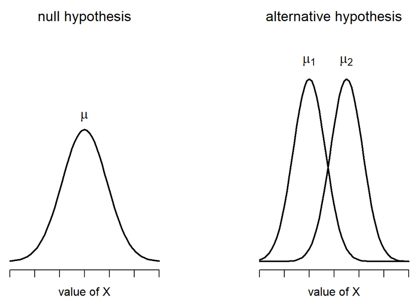
Student’s t-test
\[ H_0 : \mu_1 = \mu_2 \ \ H_1 : \mu_1 \neq \mu_2 \]
Student’s t-test: Calculate SE
Are able to use a pooled variance estimate
Both variances/standard deviations are assumed to be equal
Therefore:
\[ SE(\bar{X_1} - \bar{X_2}) = \hat{\sigma} \sqrt{\frac{1}{N_1} + \frac{1}{N_2}} \]
We are calculating the Standard Error of the Difference between means
Degrees of Freedom: Total N - 2
Student’s t-test
Let’s try it out using the traditional t.test() function
    Two Sample t-test

data:  Sleep_Hours_Schoolnight by Region
t = -0.023951, df = 180, p-value = 0.9809
alternative hypothesis: true difference in means between group NM and group NY is not equal to 0
95 percent confidence interval:
 -0.4281648  0.4178954
sample estimates:
mean in group NM mean in group NY
        6.989247         6.994382
Student’s t-test: Write-up
The mean amount of sleep in New Mexico for youth was 6.989 (SD = 1.379), while the mean in New York was 6.994 (SD = 1.512). A Student’s independent samples t-test showed that there was not a significant mean difference (t(180)=-0.024, p=.981, \(CI_{95}\)=[-0.43, 0.42], d=.004). This suggests that there is no difference between youth in NM and NY on amount of sleep on school nights.
Welch’s t-test
\[ H_0 : \mu_1 = \mu_2 \ \ H_1 : \mu_1 \neq \mu_2 \]
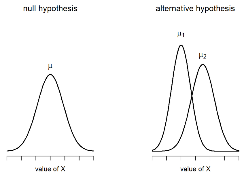
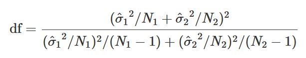
Welch’s t-test: Calculate SE
Since the variances are not equal, we have to estimate the SE differently
\[ SE(\bar{X_1} - \bar{X_2}) = \sqrt{\frac{\hat{\sigma_1^2}}{N_1} + \frac{\hat{\sigma_2^2}}{N_2}} \]
Degrees of Freedom is also very different:
Welch’s t-test: In R (classic)
Let’s try it out using the traditional t.test() function…turns out it is pretty straightforward
    Welch Two Sample t-test

data:  Sleep_Hours_Schoolnight by Region
t = -0.023902, df = 176.74, p-value = 0.981
alternative hypothesis: true difference in means between group NM and group NY is not equal to 0
95 percent confidence interval:
 -0.4290776  0.4188082
sample estimates:
mean in group NM mean in group NY
        6.989247         6.994382
Cool Visualizations
The library ggstatsplot has some wonderful visualizations of various tests
