Unit 7 - ANOVA & regression

PSYC 640 - Fall 2024

Dustin Haraden, PhD

Reminders

  • Journal Entries
  • Register to Vote
  • Presentation #2
  • Grading to be done this week (sorry)
  • Mid-course Feedback

Presentation #2

  • Beginning on 10/22

  • Groups of 2-3

  • Identify a paper that performs a statistical analysis that we have (or will) talk about in class.

    • If it is outside of what we’ve talked about, reach out to me to see if it may still work
  • Describe the main question, the research design, the analysis and interpretation

  • Provide a brief reflection on the match/mismatch of research design to analytic decision as well as anything else in the paper that could bias the results

  • More structured instructions to be posted on myCourses

Last Class

  • t-tests
    • Professors presentation didn’t work, so we did more live coding (and he probably confused everyone)
    • We took a look at easystats::report()

Today…

One-Way ANOVA

Two-Way ANOVA

# File management
library(here)
# for dplyr, ggplot2
library(tidyverse)
#Loading data
library(rio)
# Estimating Marginal Means
library(emmeans)
# Pretty Tables
library(kableExtra)
# Pretty variable names
library(janitor)

#Remove Scientific Notation 
options(scipen=999)

Review of One-Way ANOVA

One-Way ANOVA

Goal: Inform of differences among the levels of our variable of interest (Omnibus Test)

Using the between and within group variance to create the \(F\)-statistic/ratio

Hypotheses:

\[ H_0: it\: is\: true\: that\: \mu_1 = \mu_2 = \mu_3 =\: ...\mu_k \\ H_1: it\: is\: \boldsymbol{not}\: true\: that\: \mu_1 = \mu_2 = \mu_3 =\: ...\mu_k \]

\(F = \frac{MS_{between}}{MS_{within}} = \frac{small}{large} < 1\)

\(F = \frac{MS_{between}}{MS_{wihin}} = \frac{large}{small} > 1\)

ANOVA table

Source of Variation df Sum of Squares Mean Squares F-statistic p-value
Group \(G-1\) \(SS_b\) \(MS_b = \frac{SS_b}{df_b}\) \(F = \frac{MS_b}{MS_w}\) \(p\)
Residual \(N-G\) \(SS_w\) \(MS_w = \frac{SS_w}{df_w}\)
Total \(N-1\) \(SS_{total}\)

One-way ANOVA

Ghost Data

Since there are 2 header rows, we need to only include the first one. To do that, we have to “skip” the first two and then give the names of the columns back to the data.

We also need to specify what the missing values are. Typically we have been working with NA which is more traditional. However, missing values in this dataset are DK/REF and a blank. This will need to be specified in the import function (used this website)

# get the names of your columns which is the first row
ghost_data_names <- read_csv(here("lectures", "data", "ghosts.csv")) %>% 
  names()

# import second time; skip row 2, and assign column names to argument col_names =
ghost_data <- read_csv(here("lectures", "data", "ghosts.csv"),
                       skip = 2,
                       col_names = ghost_data_names,
                       na = c("DK/REF", "", " ")
                      ) %>% 
  clean_names()

Running the Test

Let’s take a look at Income by Political Affiliation

aov1 <- aov(income ~ political_affiliation, 
            data = ghost_data)

summary(aov1)
                       Df        Sum Sq     Mean Sq F value Pr(>F)  
political_affiliation   2   44252069121 22126034561   4.007 0.0189 *
Residuals             393 2170016726333  5521671059                 
---
Signif. codes:  0 '***' 0.001 '**' 0.01 '*' 0.05 '.' 0.1 ' ' 1
604 observations deleted due to missingness

Post-hoc tests

#get basic summary stats
ghost_data %>% 
  group_by(political_affiliation) %>% 
  summarise(mean = mean(income, na.rm = TRUE), 
            sd = sd(income, na.rm = TRUE))
# A tibble: 4 × 3
  political_affiliation    mean     sd
  <chr>                   <dbl>  <dbl>
1 Democrat               80431. 73147.
2 Independent           103919. 87848.
3 Republican             85623. 49064.
4 <NA>                   78233. 51022.
# conduct the comparisons
emmeans(aov1, pairwise ~ political_affiliation, 
        adjust = "none")
$emmeans
 political_affiliation emmean   SE  df lower.CL upper.CL
 Democrat               80431 6520 393    67618    93244
 Independent           103919 5870 393    92369   115468
 Republican             85623 7220 393    71433    99812

Confidence level used: 0.95 

$contrasts
 contrast                 estimate   SE  df t.ratio p.value
 Democrat - Independent     -23488 8770 393  -2.677  0.0077
 Democrat - Republican       -5192 9720 393  -0.534  0.5937
 Independent - Republican    18296 9310 393   1.966  0.0500

Family-wise error

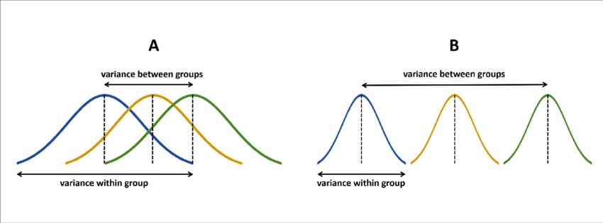
These pairwise comparisons can quickly grow in number as the number of Groups increases. With 3 (k) Groups, we have k(k-1)/2 = 3 possible pairwise comparisons.

As the number of groups in the ANOVA grows, the number of possible pairwise comparisons increases dramatically.

As the number of tests grows, and assuming the null hypothesis is true, the probability that we will make one or more Type I errors increases. To approximate the magnitude of the problem, we can assume that the multiple pairwise comparisons are independent. The probability that we don’t make a Type I error for one test is:

\[P(\text{No Type I}, 1 \text{ test}) = 1-\alpha\]

The probability that we don’t make a Type I error for two tests is:

\[P(\text{No Type I}, 2 \text{ test}) = (1-\alpha)(1-\alpha)\]

For C tests, the probability that we make no Type I errors is

\[P(\text{No Type I}, C \text{ tests}) = (1-\alpha)^C\]

We can then use the following to calculate the probability that we make one or more Type I errors in a collection of C independent tests.

\[P(\text{At least one Type I}, C \text{ tests}) = 1-(1-\alpha)^C\]

The Type I error inflation that accompanies multiple comparisons motivates the large number of “correction” procedures that have been developed.

Multiple comparisons, each tested with \(\alpha_{per-test}\), increases the family-wise \(\alpha\) level.

\[\large \alpha_{family-wise} = 1 - (1-\alpha_{per-test})^C\] Šidák showed that the family-wise a could be controlled to a desired level (e.g., .05) by changing the \(\alpha_{per-test}\) to:

\[\large \alpha_{per-wise} = 1 - (1-\alpha_{family-wise})^{\frac{1}{C}}\]

Bonferroni

Bonferroni (and Dunn, and others) suggested this simple approximation:

\[\large \alpha_{per-test} = \frac{\alpha_{family-wise}}{C}\]

This is typically called the Bonferroni correction and is very often used even though better alternatives are available.

emmeans(aov1, pairwise ~ political_affiliation, 
        adjust = "bonferroni")
$emmeans
 political_affiliation emmean   SE  df lower.CL upper.CL
 Democrat               80431 6520 393    67618    93244
 Independent           103919 5870 393    92369   115468
 Republican             85623 7220 393    71433    99812

Confidence level used: 0.95 

$contrasts
 contrast                 estimate   SE  df t.ratio p.value
 Democrat - Independent     -23488 8770 393  -2.677  0.0232
 Democrat - Republican       -5192 9720 393  -0.534  1.0000
 Independent - Republican    18296 9310 393   1.966  0.1500

P value adjustment: bonferroni method for 3 tests 

The Bonferroni procedure is conservative. Other correction procedures have been developed that control family-wise Type I error at .05 but that are more powerful than the Bonferroni procedure. The most common one is the Holm procedure.

The Holm procedure does not make a constant adjustment to each per-test \(\alpha\). Instead it makes adjustments in stages depending on the relative size of each pairwise p-value.

Holm correction

  1. Rank order the p-values from largest to smallest.
  2. Start with the smallest p-value. Multiply it by its rank.
  3. Go to the next smallest p-value. Multiply it by its rank. If the result is larger than the adjusted p-value of next smallest rank, keep it. Otherwise replace with the previous step adjusted p-value.
  4. Repeat Step 3 for the remaining p-values.
  5. Judge significance of each new p-value against \(\alpha = .05\).
Original p value Rank Rank x p Holm Bonferroni
0.0012 6 0.0072 0.0072 0.0072
0.0023 5 0.0115 0.0115 0.0138
0.0450 4 0.1800 0.1800 0.2700
0.0470 3 0.1410 0.1800 0.2820
0.0530 2 0.1060 0.1800 0.3180
0.2100 1 0.2100 0.2100 1.0000
emmeans(aov1, pairwise ~ political_affiliation, 
        adjust = "holm")
$emmeans
 political_affiliation emmean   SE  df lower.CL upper.CL
 Democrat               80431 6520 393    67618    93244
 Independent           103919 5870 393    92369   115468
 Republican             85623 7220 393    71433    99812

Confidence level used: 0.95 

$contrasts
 contrast                 estimate   SE  df t.ratio p.value
 Democrat - Independent     -23488 8770 393  -2.677  0.0232
 Democrat - Republican       -5192 9720 393  -0.534  0.5937
 Independent - Republican    18296 9310 393   1.966  0.1000

P value adjustment: holm method for 3 tests 

ANOVA is regression

In regression, we can accommodate categorical predictors. How does this compare to ANOVA?

  • Same omnibus test of the model!

*(Really the same model, but packaged differently.)

  • When would you use one versus the other?

ANOVA

  • More traditional for 3+ groups

  • Comparing/controlling multiple categorical variables

Regression

  • Best for two groups

  • Incorporating continuous predictors too

  • Good for 3+ groups when you have more specific hypotheses (contrasts)

Two-Way ANOVA

What is a Two-Way ANOVA?

Examines the impact of 2 nominal/categorical variables on a continuous outcome

We can now examine:

  • The impact of variable 1 on the outcome (Main Effect)

  • The impact of variable 2 on the outcome (Main Effect)

  • The interaction of variable 1 & 2 on the outcome (Interaction Effect)

    • The effect of variable 1 depends on the level of variable 2

Main Effect & Interactions

Main Effect: Basically a one-way ANOVA

  • The effect of variable 1 is the same across all levels of variable 2

Interaction:

  • Able to examine the effect of variable 1 across different levels of variable 2

  • Basically speaking, the effect of variable 1 on our outcome DEPENDS on the levels of variable 2

Example Data

Data

We are interested on the impact of phone usage on overall sleep quality

We include 2 variables of interest: 1) Phone Type (iOS vs. Android) and 2) Amount of usage (High, Medium & Low) to examine if there are differences in terms of sleep quality

Note: It is important to consider HOW we operationalize constructs as some things we have as factors could easily be continuous variables

Code
#Generate some data

# Set random seed for reproducibility
set.seed(42)

n <- 500  # Set number of observations

# Generate Type of Phone data
phone_type <- sample(c("Android", "iOS"), 
                     n, 
                     replace = TRUE)

# Generate Phone Usage data
phone_usage <- factor(sample(c("Low", "Medium", "High"), 
                             n, 
                             replace = TRUE), 
                      levels= c("Low", "Medium", "High"))

# Generate Sleep Quality data (with some variation)
# Intentionally inflating to highlight main effects
sleep_quality <- round(
  rnorm(n, mean = ifelse(phone_type == "Android", 5, 7) + ifelse(phone_usage == "High", 1, -1), sd = 1),
  1
)

# Generate Sleep Quality data (with some variation)
sleep_quality2 <- round(rnorm(n, mean = 6, sd = 3),1)

# Create a data frame
sleep_data <- data.frame(phone_type, 
                         phone_usage, 
                         sleep_quality,
                         sleep_quality2)

head(sleep_data)
  phone_type phone_usage sleep_quality sleep_quality2
1    Android        High           5.0           12.5
2    Android         Low           3.8           12.8
3    Android      Medium           3.9            8.7
4    Android      Medium           3.3            5.8
5        iOS         Low           5.6            8.0
6        iOS        High           7.8            3.6

Test Statistics

We’ve gone too far today without me showing some equations

With one way anova, we calculated the \(SS_{between}\) and the \(SS_{within}\) and were able to use those to capture the F-statistic

Now we have another variable to take into account. Therefore, we need to calculate:

\[ SS_{between Group1}, \: SS_{between Group2} \]

\[ SS_{within}, \: SS_{total} \]

\(F\)-Statistic/Ratio

Helpful site for hand calculations: (link)

  • Since we have these various sum of squares, we can then fill out the ANOVA table

  • This also means that we will have multiple F-Statistics

Source of Variation df Sum of Squares Mean Squares F-statistic p-value
Group1 \(j-1\) \(SS_{b1}\) \(MS_{b1} = \frac{SS_{b1}}{df_{b1}}\) \(F_1 = \frac{MS_{b1}}{MS_{w1}}\) \(p_1\)
Group2 \(k-1\) \(SS_{b2}\) \(MS_{b2} = \frac{SS_{b2}}{df_{b2}}\) \(F_2 = \frac{MS_{b2}}{MS_{w2}}\) \(p_2\)
Interaction \(df_1*df_2\)

\(SS_{int}\)

\(MS_{b3} = \frac{SS_{b3}}{df_{b3}}\) \(F_2 = \frac{MS_{b3}}{MS_{w3}}\) \(p_3\)
Residual (within) \(N-G\) \(SS_w\) \(MS_w = \frac{SS_w}{df_w}\)
Total \(N-1\) \(SS_{total}\)

Calculate \(SS_{interaction}\)

Now we need to be able to take into account the interaction term

This is done by calculating all other \(SS\) and then performing:

\[ SS_{interaction} = SS_{total} - SS_{b1} - SS_{b2} - SS_{w} \]

Example: Calculate the \(SS\) for the new data

  • no…we aren’t doing that

Running in R

Take a peak at the dataset again so we can look at the variables and their names

head(sleep_data)
  phone_type phone_usage sleep_quality sleep_quality2
1    Android        High           5.0           12.5
2    Android         Low           3.8           12.8
3    Android      Medium           3.9            8.7
4    Android      Medium           3.3            5.8
5        iOS         Low           5.6            8.0
6        iOS        High           7.8            3.6

Running in R

We will use the aov() function to set up our model

fit2 <- aov(sleep_quality ~ phone_type + phone_usage + phone_type*phone_usage, 
            data = sleep_data)

#OR 

fit2 <- aov(sleep_quality ~ phone_type * phone_usage, 
            data = sleep_data)

summary(fit2)
                        Df Sum Sq Mean Sq F value              Pr(>F)    
phone_type               1  544.6   544.6 515.727 <0.0000000000000002 ***
phone_usage              2  498.7   249.4 236.148 <0.0000000000000002 ***
phone_type:phone_usage   2    0.7     0.3   0.317               0.728    
Residuals              494  521.6     1.1                                
---
Signif. codes:  0 '***' 0.001 '**' 0.01 '*' 0.05 '.' 0.1 ' ' 1
Code
ggplot(sleep_data, aes(x = phone_usage, 
                       y = sleep_quality, 
                       color = phone_type, 
                       group = phone_type)) +
  geom_point() +
  geom_smooth(method = "lm",
              se=FALSE) +
  labs(x = "Phone Usage", 
       y = "Sleep Quality", 
       color = "Phone Type") +
  theme_minimal()

Different Outcome

Created the outcome of sleep_quality2 to be completely random instead of following a formula so that we could visualize the effect

fit3 <- aov(sleep_quality2 ~ phone_type * phone_usage, 
            data = sleep_data)
summary(fit3)
                        Df Sum Sq Mean Sq F value Pr(>F)   
phone_type               1     86   85.65   9.162 0.0026 **
phone_usage              2     56   27.83   2.977 0.0519 . 
phone_type:phone_usage   2      8    4.18   0.447 0.6399   
Residuals              494   4618    9.35                  
---
Signif. codes:  0 '***' 0.001 '**' 0.01 '*' 0.05 '.' 0.1 ' ' 1
# Create an interaction plot using ggplot2
ggplot(sleep_data, aes(x = phone_usage, y = sleep_quality2, color = phone_type, group = phone_type)) +
  geom_point() +
  geom_smooth(method = "lm",
              se=FALSE) +
  labs(x = "Phone Usage", y = "Sleep Quality", color = "Phone Type") +
  theme_minimal()

Regression

Today…

Regression

  • Why use regression?

  • One equation to rule them all

Today…

Regression

  • Why use regression?

  • One equation to rule them all

    • Ordinary Least Squares

    • Interpretation

#Don't know if I'm using all of these, but including theme here anyways
library(tidyverse)
library(rio)
library(broom)
library(psych)
library(gapminder)
library(psychTools)


#Remove Scientific Notation 
options(scipen=999)

Overview of Regression

Regression is a general data analytic system

  • Lots of things fall under the umbrella of regression

  • This system can handle a variety of forms of relations and types of variables

The output of regression includes both effect sizes and statistical significance

We can also incorporate multiple influences (IVs) and account for their intercorrelations

Uses for regression

  • Adjustment: Take into account (control) known effects in a relationship

  • Prediction: Develop a model based on what has happened previously to predict what will happen in the future

  • Explanation: examining the influence of one or more variable on some outcome

Regression Equation

With regression, we are building a model that we think best represents the data at hand

At the most simple form we are drawing a line to characterize the linear relationship between the variables so that for any value of x we can have an estimate of y

\[ Y = mX + b \]

  • Y = Outcome Variable (DV)

  • m = Slope Term

  • X = Predictor (IV)

  • b = Intercept

Regression Equation

Overall, we are providing a model to give us a “best guess” on predicting

Let’s “science up” the equation a little bit:

\[ Y_i = b_0 + b_1X_i + e_i \]

This equation is capturing how we are able to calculate each observation ( \(Y_i\) )

\[ \hat{Y_i} = b_0 + b_1X_i \]

This one will give us the “best guess” or expected value of \(Y\) given \(X\)

Regression Equation

There are two ways to think about our regression equation. They’re similar to each other, but they produce different outputs.
\[Y_i = b_{0} + b_{1}X_i +e_i\]
\[\hat{Y_i} = b_{0} + b_{1}X_i\]
The model we are building by including new variables is to explain variance in our outcome

Expected vs. Actual

\[Y_i = b_{0} + b_{1}X_i + e_i\]

\[\hat{Y_i} = b_{0} + b_{1}X_i\]

\(\hat{Y}\) signifies that there is no error. Our line is predicting that exact value. We interpret it as being “on average”

Important to identify that that \(Y_i - \hat{Y_i} = e_i\).

OLS

  • How do we find the regression estimates?

  • Ordinary Least Squares (OLS) estimation

  • Minimizes deviations

    • \[ min\sum(Y_{i} - \hat{Y} ) ^{2} \]
  • Other estimation procedures possible (and necessary in some cases)

Code
set.seed(142)
x.1 <- rnorm(10, 0, 1)
e.1 <- rnorm(10, 0, 2)
y.1 <- .5 + .55 * x.1 + e.1
d.1 <- data.frame(x.1,y.1)
m.1 <- lm(y.1 ~ x.1, data = d.1)
d1.f<- augment(m.1)


ggplot(d1.f , aes(x=x.1, y=y.1)) +
    geom_point(size = 2) +
  geom_smooth(method = lm, se = FALSE) +
  theme_bw(base_size = 20)
Code
ggplot(d1.f , aes(x=x.1, y=y.1)) +
    geom_point(size = 2) +
  geom_point(aes(y = .fitted), shape = 1, size = 2) +
  theme_bw(base_size = 20)
Code
ggplot(d1.f , aes(x=x.1, y=y.1)) +
    geom_point(size = 2) +
  geom_point(aes(y = .fitted), shape = 1, size = 2) +
  geom_segment(aes( xend = x.1, yend = .fitted))+
  theme_bw(base_size = 20)
Code
ggplot(d1.f , aes(x=x.1, y=y.1)) +
    geom_point(size = 2) +
  geom_smooth(method = lm, se = FALSE) +
  geom_point(aes(y = .fitted), shape = 1, size = 2) +
  geom_segment(aes( xend = x.1, yend = .fitted))+
  theme_bw(base_size = 20)

compare to bad fit

OLS

The line that yields the smallest sum of squared deviations

\[\Sigma(Y_i - \hat{Y_i})^2\] \[= \Sigma(Y_i - (b_0+b_{1}X_i))^2\] \[= \Sigma(e_i)^2\]

In order to find the OLS solution, you could try many different coefficients \((b_0 \text{ and } b_{1})\) until you find the one with the smallest sum squared deviation. Luckily, there are simple calculations that will yield the OLS solution every time.

Regression coefficient, \(b_{1}\)

\[b_{1} = \frac{cov_{XY}}{s_{x}^{2}} = r_{xy} \frac{s_{y}}{s_{x}}\]

What units is the regression coefficient in?

The regression coefficient (slope) equals the estimated change in Y for a 1-unit change in X

\[\Large b_{1} = r_{xy} \frac{s_{y}}{s_{x}}\]

If the standard deviation of both X and Y is equal to 1:

\[\Large b_1 = r_{xy} \frac{s_{y}}{s_{x}} = r_{xy} \frac{1}{1} = r_{xy} = \beta_{yx} = b_{yx}^*\]

Standardized regression equation

\[\Large Z_{y_i} = b_{yx}^*Z_{x_i}+e_i\]

\[\Large b_{yx}^* = b_{yx}\frac{s_x}{s_y} = r_{xy}\]

According to this regression equation, when \(X = 0, Y = 0\). Our interpretation of the coefficient is that a one-standard deviation increase in X is associated with a \(b_{yx}^*\) standard deviation increase in Y. Our regression coefficient is equivalent to the correlation coefficient when we have only one predictor in our model.

Estimating the intercept, \(b_0\)

  • intercept serves to adjust for differences in means between X and Y

\[\hat{Y_i} = \bar{Y} + r_{xy} \frac{s_{y}}{s_{x}}(X_i-\bar{X})\]

  • if standardized, intercept drops out

  • otherwise, intercept is where regression line crosses the y-axis at X = 0

The intercept adjusts the location of the regression line to ensure that it runs through the point \(\large (\bar{X}, \bar{Y}).\) We can calculate this value using the equation:

\[\Large b_0 = \bar{Y} - b_1\bar{X}\]

Example

library(gapminder)
gapminder = gapminder %>% filter(year == 2007 & continent == "Asia") %>% 
  mutate(log_gdp = log(gdpPercap))
describe(gapminder[,c("log_gdp", "lifeExp")], fast = T)
        vars  n  mean   sd median   min   max range  skew kurtosis   se
log_gdp    1 33  8.74 1.24   8.41  6.85 10.76  3.91  0.21    -1.37 0.22
lifeExp    2 33 70.73 7.96  72.40 43.83 82.60 38.77 -1.07     1.79 1.39
cor(gapminder$log_gdp, gapminder$lifeExp)
[1] 0.8003474

If we regress lifeExp onto log_gdp:

r = cor(gapminder$log_gdp, gapminder$lifeExp)
m_log_gdp = mean(gapminder$log_gdp)
m_lifeExp = mean(gapminder$lifeExp)
s_log_gdp = sd(gapminder$log_gdp)
s_lifeExp = sd(gapminder$lifeExp)

b1 = r*(s_lifeExp/s_log_gdp)
[1] 5.157259
b0 = m_lifeExp - b1*m_log_gdp
[1] 25.65011

How will this change if we regress GDP onto life expectancy?

(b1 = r*(s_lifeExp/s_log_gdp))
[1] 5.157259
(b0 = m_lifeExp - b1*m_log_gdp)
[1] 25.65011
(b1 = r*(s_log_gdp/s_lifeExp))
[1] 0.1242047
(b0 = m_log_gdp - b1*m_lifeExp)
[1] -0.04405086

In R

fit.1 <- lm(lifeExp ~ log_gdp, data = gapminder)
summary(fit.1)

Call:
lm(formula = lifeExp ~ log_gdp, data = gapminder)

Residuals:
    Min      1Q  Median      3Q     Max 
-17.314  -1.650  -0.040   3.428   8.370 

Coefficients:
            Estimate Std. Error t value     Pr(>|t|)    
(Intercept)  25.6501     6.1234   4.189     0.000216 ***
log_gdp       5.1573     0.6939   7.433 0.0000000226 ***
---
Signif. codes:  0 '***' 0.001 '**' 0.01 '*' 0.05 '.' 0.1 ' ' 1

Residual standard error: 4.851 on 31 degrees of freedom
Multiple R-squared:  0.6406,    Adjusted R-squared:  0.629 
F-statistic: 55.24 on 1 and 31 DF,  p-value: 0.00000002263

Data, fitted, and residuals

library(broom)
model_info = augment(fit.1)
head(model_info)
# A tibble: 6 × 8
  lifeExp log_gdp .fitted .resid   .hat .sigma .cooksd .std.resid
    <dbl>   <dbl>   <dbl>  <dbl>  <dbl>  <dbl>   <dbl>      <dbl>
1    43.8    6.88    61.1 -17.3  0.101    3.63 0.796       -3.76 
2    75.6   10.3     78.8  -3.15 0.0802   4.89 0.0199      -0.676
3    64.1    7.24    63.0   1.08 0.0765   4.93 0.00224      0.233
4    59.7    7.45    64.1  -4.33 0.0646   4.86 0.0294      -0.923
5    73.0    8.51    69.5   3.43 0.0314   4.89 0.00836      0.718
6    82.2   10.6     80.3   1.94 0.100    4.92 0.00994      0.422
describe(model_info, fast = T)
           vars  n  mean   sd median    min   max range  skew kurtosis   se
lifeExp       1 33 70.73 7.96  72.40  43.83 82.60 38.77 -1.07     1.79 1.39
log_gdp       2 33  8.74 1.24   8.41   6.85 10.76  3.91  0.21    -1.37 0.22
.fitted       3 33 70.73 6.37  69.00  60.98 81.16 20.19  0.21    -1.37 1.11
.resid        4 33  0.00 4.77  -0.04 -17.31  8.37 25.68 -1.37     3.29 0.83
.hat          5 33  0.06 0.03   0.05   0.03  0.11  0.08  0.60    -0.98 0.00
.sigma        6 33  4.84 0.23   4.90   3.63  4.93  1.30 -4.53    20.90 0.04
.cooksd       7 33  0.04 0.14   0.01   0.00  0.80  0.80  5.08    25.12 0.02
.std.resid    8 33  0.00 1.02  -0.01  -3.76  1.77  5.53 -1.44     3.56 0.18

The relationship between \(X_i\) and \(\hat{Y_i}\)

Code
model_info %>% ggplot(aes(x = log_gdp, y = .fitted)) +
  geom_point() + geom_smooth(se = F, method = "lm") +
  scale_x_continuous("X") + scale_y_continuous(expression(hat(Y))) + theme_bw(base_size = 30)

The relationship between \(X_i\) and \(e_i\)

Code
model_info %>% ggplot(aes(x = log_gdp, y = .resid)) +
  geom_point() + geom_smooth(se = F, method = "lm") + 
  scale_x_continuous("X") + scale_y_continuous("e") + theme_bw(base_size = 30)

The relationship between \(Y_i\) and \(\hat{Y_i}\)

Code
model_info %>% ggplot(aes(x = lifeExp, y = .fitted)) +
  geom_point() + geom_smooth(se = F, method = "lm") + 
  scale_x_continuous("Y") + scale_y_continuous(expression(hat(Y))) + theme_bw(base_size = 30)

The relationship between \(Y_i\) and \(e_i\)

Code
model_info %>% ggplot(aes(x = lifeExp, y = .resid)) +
  geom_point() + geom_smooth(se = F, method = "lm") + 
  scale_x_continuous("Y") + scale_y_continuous("e") + theme_bw(base_size = 25)

The relationship between \(\hat{Y_i}\) and \(e_i\)

Code
model_info %>% ggplot(aes(x = .fitted, y = .resid)) +
  geom_point() + geom_smooth(se = F, method = "lm") + 
  scale_y_continuous("e") + scale_x_continuous(expression(hat(Y))) + theme_bw(base_size = 30)

Regression to the mean

An observation about heights was part of the motivation to develop the regression equation: If you selected a parent who was exceptionally tall (or short), their child was almost always not as tall (or as short).

Code
library(psychTools)
library(tidyverse)
heights = psychTools::galton
mod = lm(child~parent, data = heights)
point = 902
heights = broom::augment(mod)


heights %>%
  ggplot(aes(x = parent, y = child)) +
  geom_jitter(alpha = .3) +
  geom_hline(aes(yintercept = 72), color = "red") +
  geom_vline(aes(xintercept = 72), color = "red") +
  theme_bw(base_size = 20)

Regression to the mean

This phenomenon is known as regression to the mean. This describes the phenomenon in which an random variable produces an extreme score on a first measurement, but a lower score on a second measurement.

Regression to the mean

This can be a threat to internal validity if interventins are applied based on first measurement scores.

Example in R

Try out a linear regression on the Ghosts Data!