Week 05: Simple Regression

Date: September 24, 2026

Today…

The Linear Model — one machine, most of the course

• Why a line? (and why regression first)
• Data = Model + Error
• Where the intercept and slope come from
• Reading a slope out loud
• How well does the line fit? (\(R^2\), effect size)
• The punchline from Lab 5

# File management
library(here)
# for dplyr, ggplot2
library(tidyverse)
# Loading data
library(rio)
# tidy model output
library(broom)
# descriptives
library(psych)
# pretty tables
library(sjPlot)

#Remove Scientific Notation
options(scipen = 999)

cah <- import(here("files", "data", "CAH.csv"))

First, a confession about Lab 5

In Lab 5 you ran three things:

1. A t-test comparing two groups
2. A correlation between two continuous variables
3. An lm() — the “sneak peek” 👀

And the numbers came back the same.

That was not a bug, and it was not a coincidence.

Important

Regression is not a new test that sits next to t-tests and correlations. It is the general machine that both of them are special cases of.

Why I teach regression first

Regression is a general data analytic system

• Lots of things fall under the umbrella of regression

• It handles many forms of relations and types of variables

• The output gives you effect sizes and statistical significance

• We can add multiple predictors and account for their intercorrelations

Learn one machine well, then add parts to it. That is the whole plan for the next eight weeks.

Uses for regression

• Adjustment: Take into account (control) known effects in a relationship

• Prediction: Develop a model based on what has happened previously to predict what will happen in the future

• Explanation: Examine the influence of one or more variables on some outcome

Part 1: Building the Line

The core idea

With regression, we are building a model that we think best represents the data, and the broader world

\[ Data = Model + error \]

Every model we build for the rest of the semester is a variation on this sentence.

A line you already know

At the simplest form we draw a line to characterize the linear relationship between two variables, so that for any value of x we have an estimate of y

\[ Y = mX + b \]

• Y = Outcome Variable (DV)

• m = Slope Term

• X = Predictor (IV)

• b = Intercept

Let’s “science up” the equation

\[ Y_i = b_0 + b_1X_i + e_i \]

This captures how we calculate each observation ( \(Y_i\) )

\[ \hat{Y_i} = b_0 + b_1X_i \]

This gives the “best guess” or expected value of \(Y\) given \(X\)

Expected vs. Actual

\[Y_i = b_{0} + b_{1}X_i + e_i \qquad \hat{Y_i} = b_{0} + b_{1}X_i\]

\(\hat{Y}\) signifies the fitted score — no error. We interpret it as “on average.”

The difference between the fitted and the observed score is the residual:

\[Y_i - \hat{Y_i} = e_i\]

Note

There is a different \(e\) value for each observation in the dataset. The residual is the part of a person your model gets wrong — hold onto that, it becomes the whole story in a few weeks.

OLS

• How do we find the regression estimates?

• Ordinary Least Squares estimation

• Minimizes deviations

  • \[ min\sum(Y_{i} - \hat{Y} ) ^{2} \]

• Other estimation procedures are possible (and necessary in some cases)

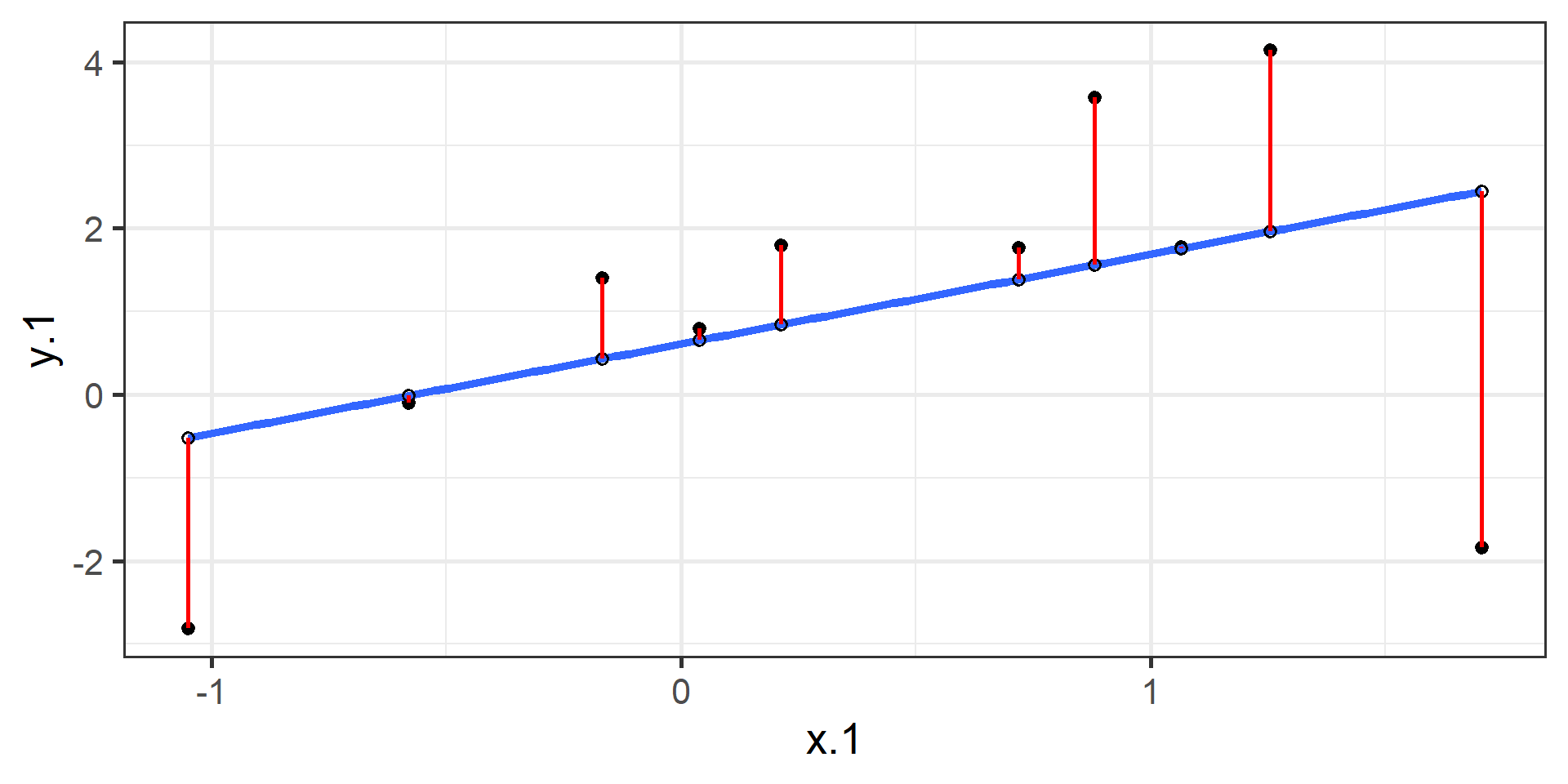
Some data

set.seed(142)
x.1 <- rnorm(10, 0, 1)
e.1 <- rnorm(10, 0, 2)
y.1 <- .5 + .55 * x.1 + e.1
d.1 <- data.frame(x.1, y.1)
m.1 <- lm(y.1 ~ x.1, data = d.1)
d1.f <- augment(m.1)

ggplot(d1.f, aes(x = x.1, y = y.1)) +
  geom_point(size = 2) +
  geom_smooth(method = lm, se = FALSE) +
  theme_bw(base_size = 20)

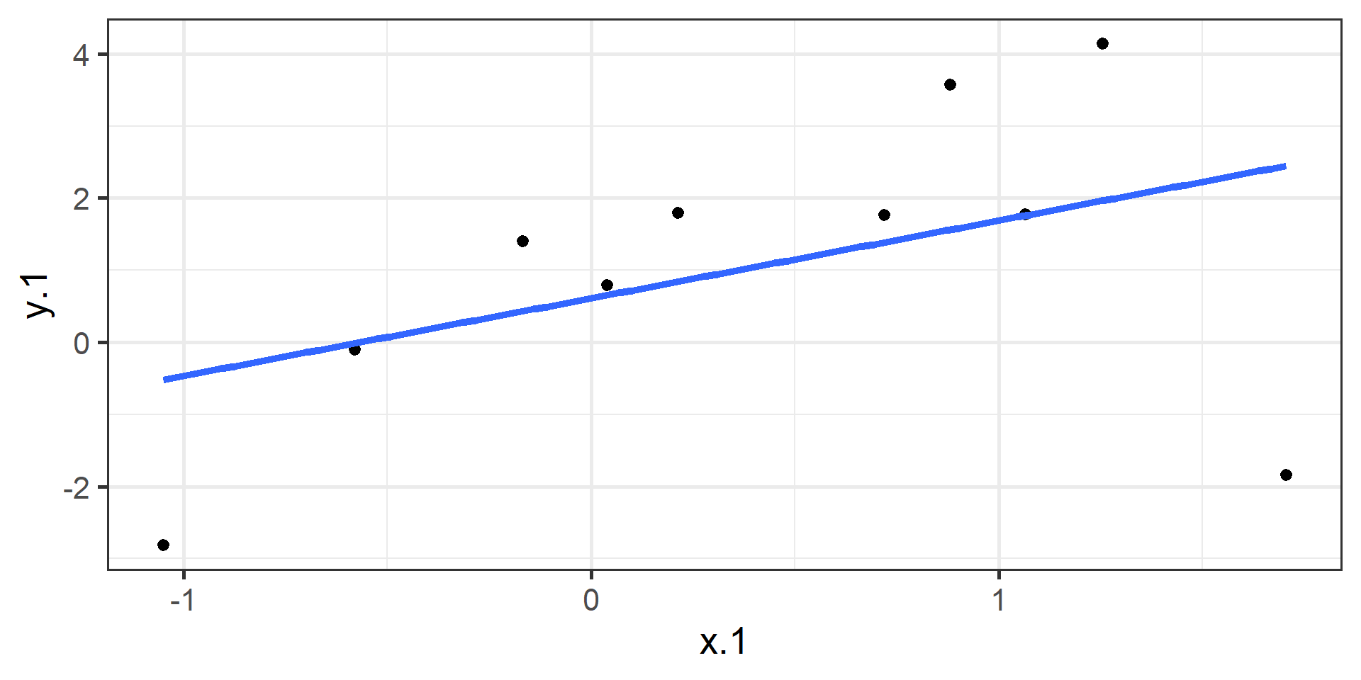
The fitted values ( \(\hat{Y}\) )

ggplot(d1.f, aes(x = x.1, y = y.1)) +
  geom_point(size = 2) +
  geom_point(aes(y = .fitted), shape = 1, size = 2) +
  theme_bw(base_size = 20)

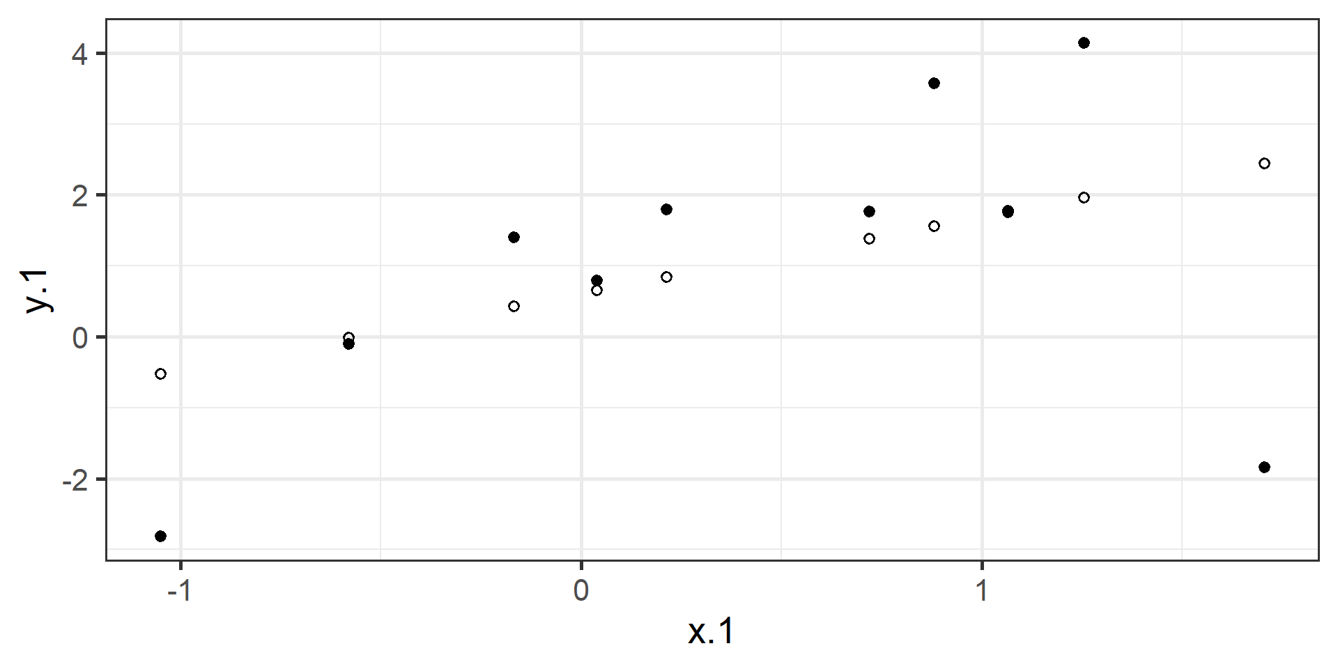
The residuals ( \(e_i\) )

ggplot(d1.f, aes(x = x.1, y = y.1)) +
  geom_point(size = 2) +
  geom_point(aes(y = .fitted), shape = 1, size = 2) +
  geom_segment(aes(xend = x.1, yend = .fitted), color = "red") +
  theme_bw(base_size = 20)

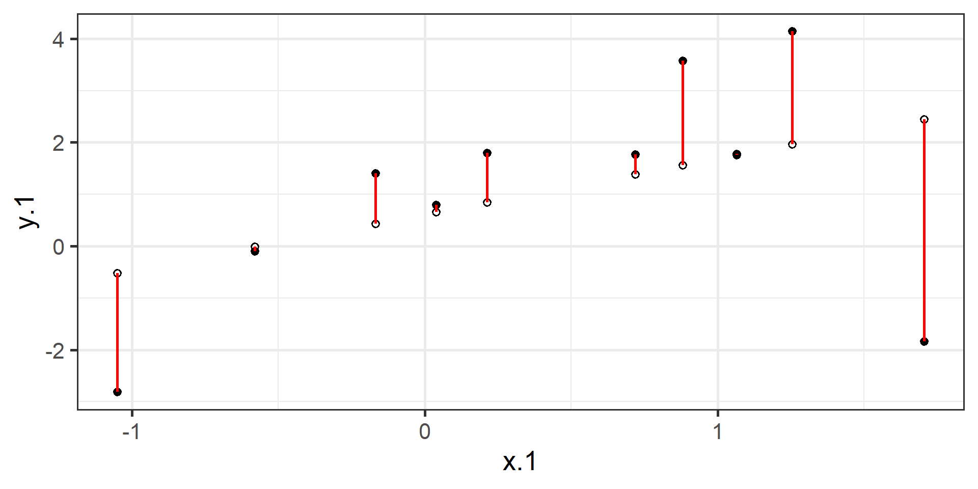
Put it together

ggplot(d1.f, aes(x = x.1, y = y.1)) +
  geom_point(size = 2) +
  geom_smooth(method = lm, se = FALSE) +
  geom_point(aes(y = .fitted), shape = 1, size = 2) +
  geom_segment(aes(xend = x.1, yend = .fitted), color = "red") +
  theme_bw(base_size = 20)

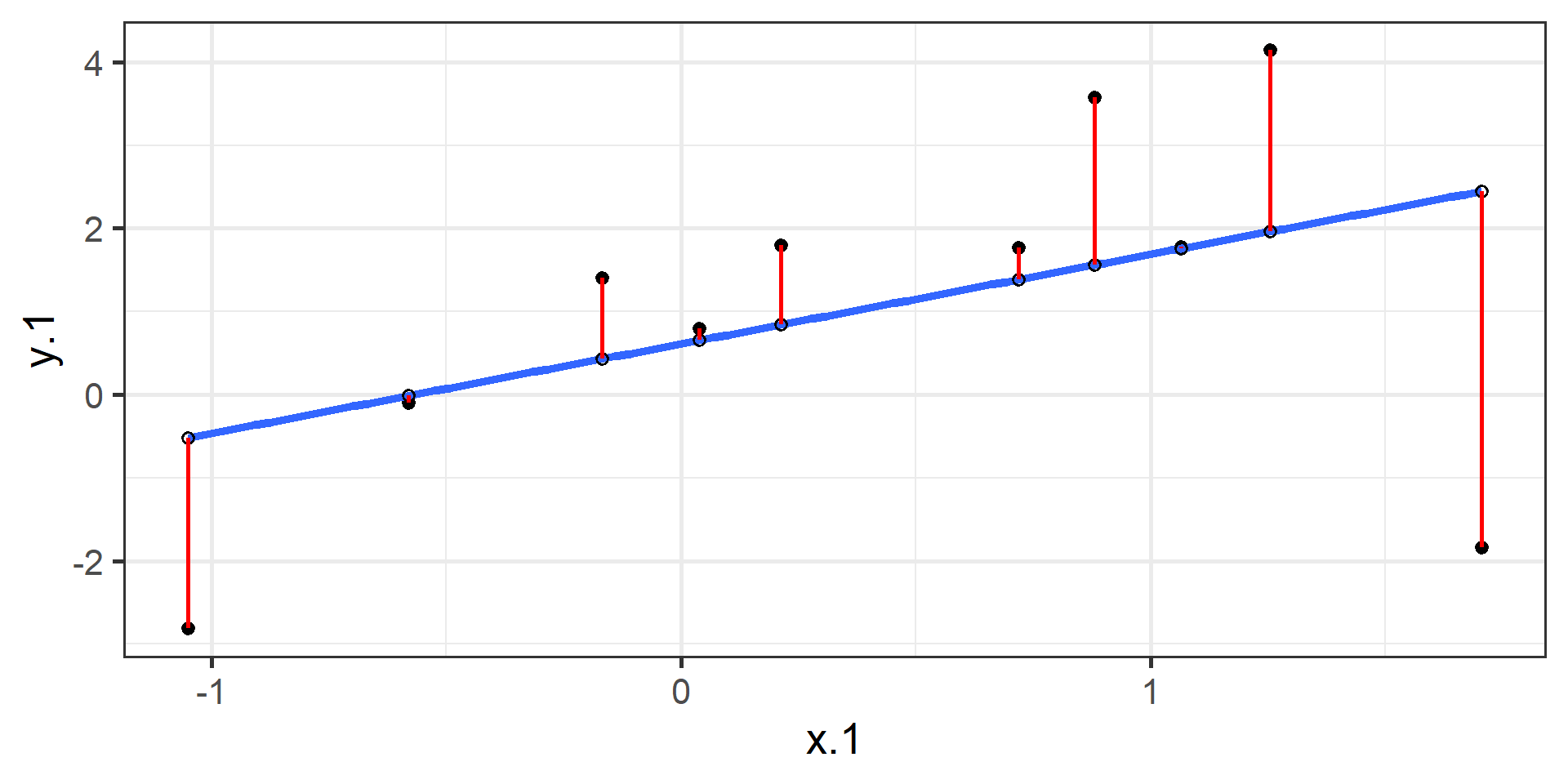
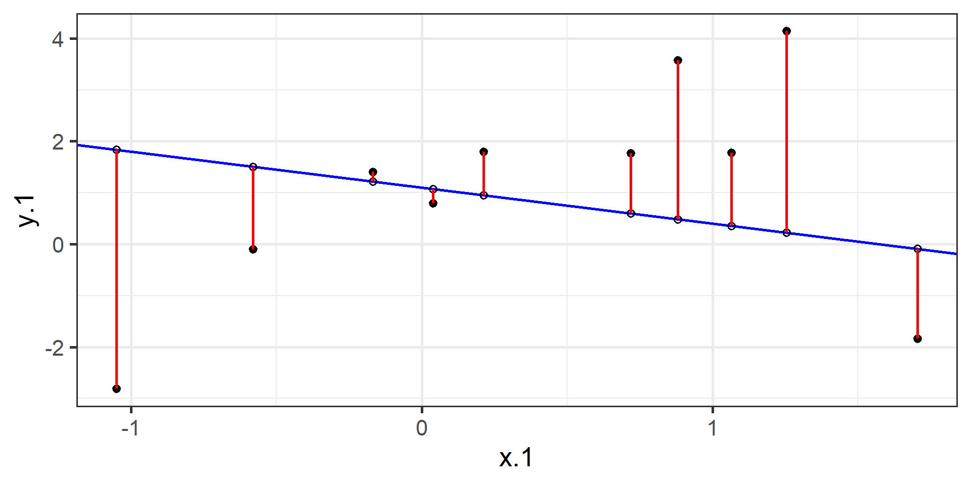
Compare to a bad fit

Which has more [RED]{style=“color: red;”}

OLS

The line that yields the smallest sum of squared deviations

\[\Sigma(Y_i - \hat{Y_i})^2\] \[= \Sigma(Y_i - (b_0+b_{1}X_i))^2\] \[= \Sigma(e_i)^2\]

You could try many different coefficients until you find the pair with the smallest sum of squared deviations. Luckily, there are simple calculations that yield the OLS solution every time.

Where does the slope come from? 🤔

Starting with the covariance between two variables:

\[cov_{xy} = \frac{\sum(x-\bar{x})(y-\bar{y})}{N-1}\]

and the correlation, which is just a standardized covariance:

\[r_{xy} = \frac{cov_{xy}}{s_x s_y}\]

The regression coefficient is built from exactly the same pieces.

Regression coefficient, \(b_{1}\)

\[b_{1} = \frac{cov_{XY}}{s_{x}^{2}} = r_{xy} \frac{s_{y}}{s_{x}}\]

What units is the regression coefficient in?

The slope equals the estimated change in Y for a 1-unit change in X

Tip

A correlation is unitless. A slope is in the units of your study. That is why a slope is often the more useful number to report to a human being.

Slope is the correlation (rescaled)

\[\Large b_{1} = r_{xy} \frac{s_{y}}{s_{x}}\]

If the standard deviation of both X and Y is equal to 1:

\[\Large b_1 = r_{xy} \frac{s_{y}}{s_{x}} = r_{xy} \frac{1}{1} = r_{xy} = \beta_{yx}\]

Standardize both variables and the slope becomes the correlation. Same information, different clothes.

Estimating the intercept, \(b_0\)

• The intercept adjusts for differences in the means of X and Y

\[\hat{Y_i} = \bar{Y} + r_{xy} \frac{s_{y}}{s_{x}}(X_i-\bar{X})\]

• It is where the regression line crosses the y-axis, at \(X = 0\)

• It ensures the line runs through the point \((\bar{X}, \bar{Y})\)

\[\Large b_0 = \bar{Y} - b_1\bar{X}\]

🔍 Visualizing OLS

Play with these — they make the “least squares” part click:

https://setosa.io/ev/ordinary-least-squares-regression/

https://observablehq.com/@yizhe-ang/interactive-visualization-of-linear-regression

Part 2: Reading a Line Out Loud

Our data today 🃏

Cards Against Humanity: Pulse of the Nation — a national poll that asked serious demographic questions and some very strange ones.

cah %>%
  select(age, transformers, books) %>%
  psych::describe()

             vars    n  mean    sd median trimmed   mad min  max range  skew
age             1 1000 49.41 16.63     50   49.30 17.79  18   99    81  0.07
transformers    2  938  1.33  1.56      1    1.10  1.48   0    5     5  0.90
books           3  977 22.33 75.87      5    9.47  7.41   0 1000  1000 10.00
             kurtosis   se
age             -0.49 0.53
transformers    -0.38 0.05
books          118.09 2.43

🛠️ Activity Stop 1: One Line, Two Stories

Tip

Part A: Follow along · ~20 min · Pairs

We fit this model together, from the top:

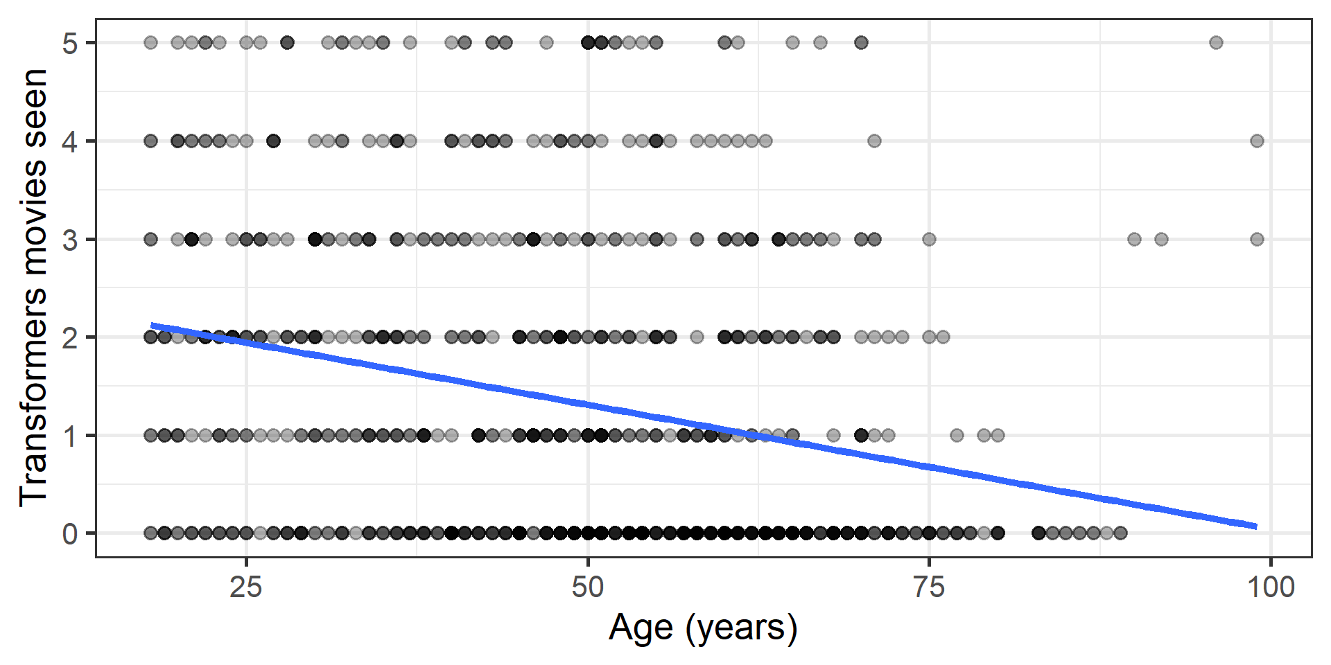
• Plot it, then guess r before you run it
• lm(), find the intercept and slope
• Say the slope in a unit that means something
• Predict a person and compute their residual

Open the activity

Step 1: ALWAYS visualize first

ggplot(cah, aes(x = age, y = transformers)) +
  geom_point(alpha = .3) +
  geom_smooth(method = "lm", se = FALSE) +
  labs(x = "Age (years)",
       y = "Transformers movies seen") +
  theme_bw(base_size = 20)

By hand, then by R

r        <- cor(cah$age, cah$transformers, use = "pairwise")
s_age    <- sd(cah$age, na.rm = TRUE)
s_tf     <- sd(cah$transformers, na.rm = TRUE)
m_age    <- mean(cah$age, na.rm = TRUE)
m_tf     <- mean(cah$transformers, na.rm = TRUE)

b1 <- r * (s_tf / s_age)
b0 <- m_tf - (b1 * m_age)

c(r = r, b1 = b1, b0 = b0)

          r          b1          b0 
-0.26644722 -0.02498682  2.56823762 

In R

fit.1 <- lm(transformers ~ age, data = cah)
summary(fit.1)

Call:
lm(formula = transformers ~ age, data = cah)

Residuals:
    Min      1Q  Median      3Q     Max 
-2.1206 -1.1055 -0.5472  0.9784  4.8588 

Coefficients:
            Estimate Std. Error t value            Pr(>|t|)    
(Intercept)  2.57733    0.15503  16.625 <0.0000000000000002 ***
age         -0.02538    0.00300  -8.457 <0.0000000000000002 ***
---
Signif. codes:  0 '***' 0.001 '**' 0.01 '*' 0.05 '.' 0.1 ' ' 1

Residual standard error: 1.504 on 936 degrees of freedom
  (62 observations deleted due to missingness)
Multiple R-squared:  0.07099,   Adjusted R-squared:   0.07 
F-statistic: 71.53 on 1 and 936 DF,  p-value: < 0.00000000000000022

Point at the Estimate column first, then the t and p. Note the slope’s t is identical to cor.test — we prove it on the next slides.

wait…they aren’t the same? Rounding?

The results are close, but not identical. What’s the deal??

c(r = r, b1 = b1, b0 = b0)

          r          b1          b0 
-0.26644722 -0.02498682  2.56823762 

tidy(fit.1)

# A tibble: 2 × 5
  term        estimate std.error statistic  p.value
  <chr>          <dbl>     <dbl>     <dbl>    <dbl>
1 (Intercept)   2.58     0.155       16.6  1.41e-54
2 age          -0.0254   0.00300     -8.46 1.04e-16

MISSING DATA

Our data has 62 participants with missing values

lm() just kicks folks out with NA - listwise deletion

Hand calculation used all participants in the data

Comparing…again

This time we are going to listwise delete participants.

cah_tf <- cah %>% drop_na(age, transformers)
r        <- cor(cah_tf$age, cah_tf$transformers, use = "pairwise")
s_age    <- sd(cah_tf$age, na.rm = TRUE)
s_tf     <- sd(cah_tf$transformers, na.rm = TRUE)
m_age    <- mean(cah_tf$age, na.rm = TRUE)
m_tf     <- mean(cah_tf$transformers, na.rm = TRUE)

b1 <- r * (s_tf / s_age)
b0 <- m_tf - (b1 * m_age)

c(r = r, b1 = b1, b0 = b0)

          r          b1          b0 
-0.26644722 -0.02537607  2.57733245 

tidy(fit.1)

# A tibble: 2 × 5
  term        estimate std.error statistic  p.value
  <chr>          <dbl>     <dbl>     <dbl>    <dbl>
1 (Intercept)   2.58     0.155       16.6  1.41e-54
2 age          -0.0254   0.00300     -8.46 1.04e-16

Saying the slope out loud

\[\widehat{transformers} = 2.58 - 0.025(age)\]

• “Each additional year of age is associated with 0.025 fewer Transformers movies seen.”

• That sounds like nothing. So rescale it to a unit people care about:

  • 10 years → about 0.25 fewer movies
  • 40 years → about one whole movie fewer

• Note the word associated. Nobody was randomly assigned an age.

And the intercept?

\(b_0 = 2.58\) = the predicted number of Transformers movies for a person aged zero.

Careful

Nobody in this sample is under 18. A prediction at age 0 is extrapolation — the model has never seen data anywhere near there.

The intercept is an anchor for the line, not a finding.

When zero is not meaningful, centering the predictor fixes the interpretation (we will do this for real in Week 9).

Predict a person

# predicted movies for a 20-year-old
b0 + b1 * 20

[1] 2.069811

A 20-year-old in the data who has seen 4 movies:

\[e_i = Y_i - \hat{Y_i} = 4 - 2.07 = +1.93\]

Positive residual → above the line → the model under-predicted this person.

☕ Break

10 minutes

When we come back: how do we know if this line is any good?

Part 3: How Well Does the Line Fit?

Statistical inference

• The way the world is = our model + error

• How good is our model? Does it “fit” the data well?

To assess fit, we examine the proportion of variance in our outcome that is “explained” by our model.

To do that, we partition the variance into two categories: variability captured by the model, and variability that is not.

Partitioning variation

Start with the relationship between observed \(Y\) and fitted \(\hat{Y}\):

\[Y_i = \hat{Y}_i + e_i\]

Variances are additive when two variables are independent. If C = A + B, then the variance of C is the sum of the variances of A and B.

Why can we use that rule here?

Students must recognize that Y-hat and e are uncorrelated — they must be, by the way OLS is built.

Partitioning variation

\(\hat{Y}_i\) and \(e_i\) are independent of each other. So the variance of \(Y\) equals the variance of \(\hat{Y}\) plus the variance of \(e\).

\[\large s^2_Y = s^2_{\hat{Y}} + s^2_{e}\]

Variances are sums of squares divided by N−1, and all have the same sample size here, so:

\[\large SS_Y = SS_{\hat{Y}} + SS_{\text{e}}\]

\[ SS_Y = SS_{\text{Model}} + SS_{\text{Residual}}\]

Coefficient of Determination

\[\Large \frac{SS_{Model}}{SS_{Y}} = \frac{s_{Model}^2}{s_{y}^2} = R^2\]

\(R^2\) is the proportion of variance in Y explained by the model

\[\large \sqrt{R^2} = r_{Y\hat{Y}}\]

With one predictor, that is just our old friend \(r\).

Ta da! 🎉

# the correlation, squared
cor(cah$age, cah$transformers, use = "pairwise")^2

[1] 0.07099412

# R-squared straight from the model
summary(fit.1)$r.squared

[1] 0.07099412

And the t for the slope?

tidy(fit.1)

# A tibble: 2 × 5
  term        estimate std.error statistic  p.value
  <chr>          <dbl>     <dbl>     <dbl>    <dbl>
1 (Intercept)   2.58     0.155       16.6  1.41e-54
2 age          -0.0254   0.00300     -8.46 1.04e-16

cor.test(cah$age, cah$transformers)$statistic

        t 
-8.457459 

Significance \(\neq\) importance

The \(p\)-value tells us the effect is likely not zero. It says nothing about whether the effect is large or meaningful.

Important

With a large enough sample, a tiny, trivial effect becomes statistically significant. Our n here is 938.

Statistical Significance \(\neq\) Practical Significance

Effect size for a regression

1. The slope itself — in the units of your study. The most concrete thing you have.

2. Standardized slope — in SD units. Cohen’s rough guide: small (|.10|), medium (|.30|), large (|.50|)

3. Coefficient of determination \(R^2\) — proportion of variance accounted for

For our model: \(r = -.27\), so \(R^2 = .071\)

“Approximately 7% of the variability in Transformers movies seen is accounted for by age.”

Writing it up

Template: b = slope, t(df) = statistic, p = p-value, plus \(R^2\)

Age significantly predicted the number of Transformers movies a respondent had seen (b = −0.03, p < .001). Each additional decade of age was associated with about a quarter of a movie fewer, and age accounted for 7.1% of the variance in movies seen (\(R^2\) = .07).

Tip

Notice what the good version includes: the estimate in real units, the test, and a statement of how much it matters. All three.

Some folks will include the t-values, but I find that overwhelming. Just have that in the tables.

Pretty tables with sjPlot

tab_model(fit.1, show.std = TRUE)

	transformers
Predictors	Estimates	std. Beta	CI	standardized CI	p
(Intercept)	2.58	0.00	2.27 – 2.88	-0.06 – 0.06	<0.001
age	-0.03	-0.27	-0.03 – -0.02	-0.33 – -0.20	<0.001
Observations	938
R2 / R2 adjusted	0.071 / 0.070

Data, fitted, and residuals

model_info <- augment(fit.1)
head(model_info)

# A tibble: 6 × 9
  .rownames transformers   age .fitted  .resid    .hat .sigma .cooksd .std.resid
  <chr>            <int> <int>   <dbl>   <dbl>   <dbl>  <dbl>   <dbl>      <dbl>
1 1                    1    64   0.953  0.0467 0.00196   1.50 9.51e-7     0.0311
2 2                    0    56   1.16  -1.16   0.00126   1.50 3.74e-4    -0.769 
3 3                    0    63   0.979 -0.979  0.00185   1.50 3.92e-4    -0.651 
4 4                    0    48   1.36  -1.36   0.00107   1.50 4.38e-4    -0.904 
5 5                    1    32   1.77  -0.765  0.00222   1.50 2.88e-4    -0.509 
6 6                    0    64   0.953 -0.953  0.00196   1.50 3.95e-4    -0.635 

Point out that the average of the residuals is 0 — just like the average deviation from the mean is 0.

The relationship between \(\hat{Y_i}\) and \(e_i\)

model_info %>%
  ggplot(aes(x = .fitted, y = .resid)) +
  geom_point(alpha = .3) +
  geom_smooth(se = F, method = "lm") +
  scale_y_continuous("e") +
  scale_x_continuous(expression(hat(Y))) +
  theme_bw(base_size = 25)

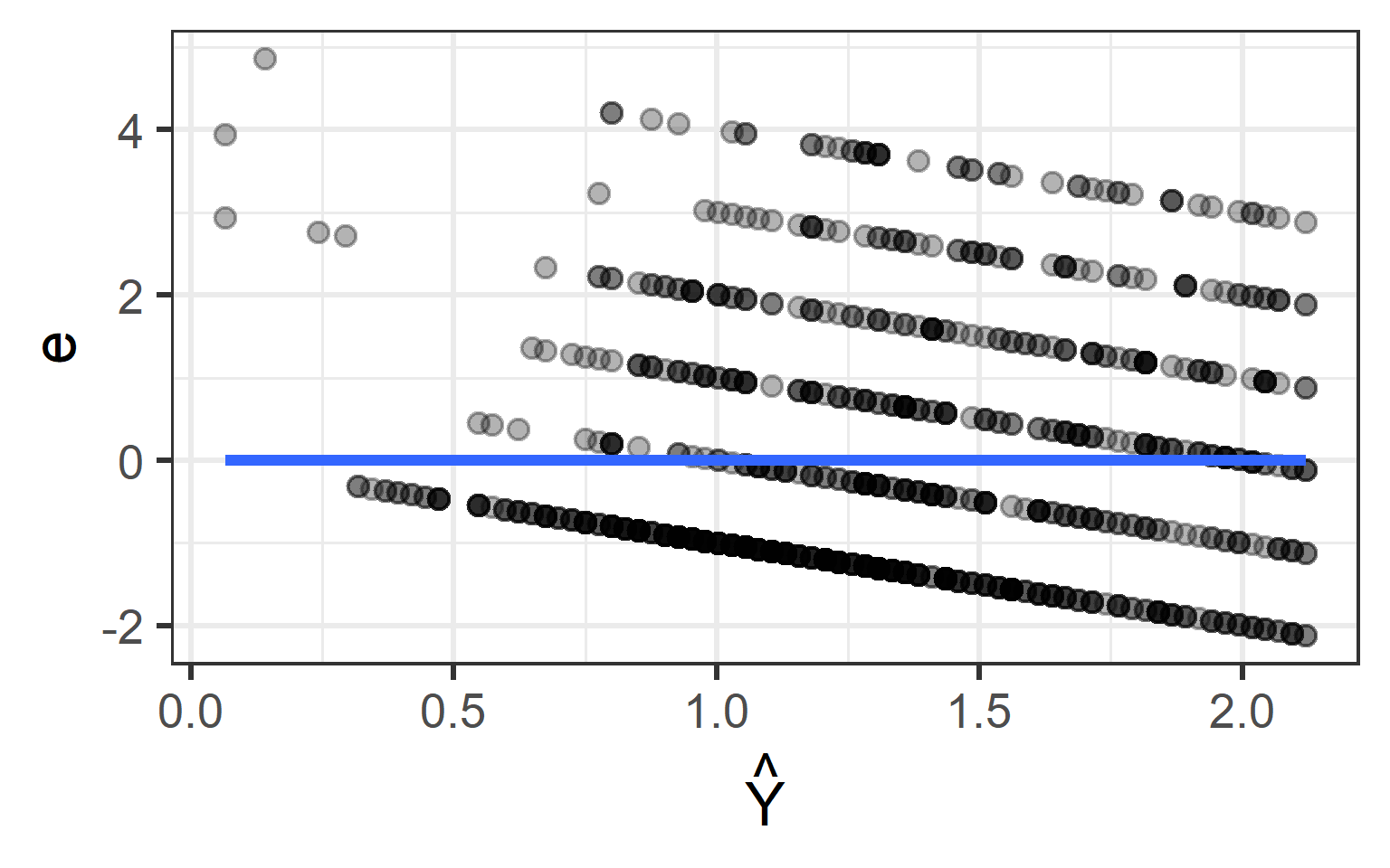
Flat. Always. By construction — and in Week 10 we will use that fact to catch models that are lying to us.

Part 4: The Lab 5 Punchline

A t-test is a regression

cah_mf <- cah %>% filter(gender == "Male" | 
                           gender == "Female") 
#OR

cah_mf <- cah %>% filter(gender %in% c("Male", "Female"))


t.test(transformers ~ gender, data = cah_mf, var.equal = TRUE)

    Two Sample t-test

data:  transformers by gender
t = -2.2886, df = 911, p-value = 0.02233
alternative hypothesis: true difference in means between group Female and group Male is not equal to 0
95 percent confidence interval:
 -0.4348223 -0.0333445
sample estimates:
mean in group Female   mean in group Male 
            1.206897             1.440980 

The same question as a line

lm(transformers ~ gender, data = cah_mf) %>% tidy()

# A tibble: 2 × 5
  term        estimate std.error statistic  p.value
  <chr>          <dbl>     <dbl>     <dbl>    <dbl>
1 (Intercept)    1.21     0.0717     16.8  1.59e-55
2 genderMale     0.234    0.102       2.29 2.23e- 2

• The intercept (1.21) is the mean of the first group (Female)
• The slope (0.23) is the difference between the means
• Same t. Same p. One machine.

Why this matters

Note

You do not have to memorize a separate procedure for every design.

outcome ~ predictor handles the continuous case and the group case. Over the next few weeks we just add more predictors to the same machine.

Next week: groups as regression, in full — t-tests and ANOVA as lm().

One more thing: regression to the mean

An observation about heights motivated the development of regression: if you selected an exceptionally tall (or short) parent, their child was almost always less extreme.

library(psychTools)
heights <- psychTools::galton
mod <- lm(child ~ parent, data = heights)
heights <- broom::augment(mod)

heights %>%
  ggplot(aes(x = parent, y = child)) +
  geom_jitter(alpha = .3) +
  geom_smooth(method = "lm", se = FALSE) +
  geom_hline(aes(yintercept = 72), color = "red") +
  geom_vline(aes(xintercept = 72), color = "red") +
  theme_bw(base_size = 20)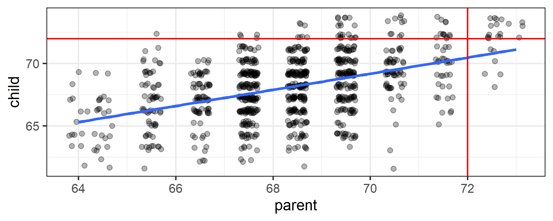

Regression to the mean

Regression to the mean: a random variable that produces an extreme score on a first measurement tends to produce a less extreme score on a second measurement.

Warning

This is a threat to internal validity whenever an intervention is assigned based on first-measurement scores.

Tutoring the students who bombed the midterm? They would have improved somewhat anyway.

🛠️ Activity Stop 2: Parts B & C

Tip

One Line, Two Stories · ~35 min · Pairs

Part B (~25 min): Do older people read more books?

• You will get p = .027 — and then one person who reported reading 1,000 books will make it disappear
• The p-value flips on a judgment call you make

Part C (~10 min): The t-test / regression equivalence, in your own file

Open the activity

✍️ Wrap-Up

Finish these at the bottom of your activity file:

1. A slope, stated in the units of a study, without using the word “slope.”
2. One intercept from today that is meaningless, and why.
3. One thing that is still muddy → put it in your journal this week.

For next time

📋 Lab 6 — Reading the Line

• Almost no coding. I give you the output; you tell me what it means.
• Uses the Lab 5 data plus a new context

📖 Chapter 15 — ST

Schedule change

The lab schedule has moved up from the PDF syllabus. Website = current version.