Week 06: Comparing Groups with JAMOVI
Date: October 1, 2026
Today…
Groups, as lines
- Why a t-test is a regression (we prove it properly this time)
- Dummy coding: how software turns a group into a number
- Three or more groups: ANOVA is the same machine
- Why not just run a bunch of t-tests?
- Effect size: d, R², and which one to report
Note
This is the JAMOVI version. Same data, same numbers, same conclusions as the R deck — only the buttons change.
Where we left off
Last week, in Part C of the activity:
- You ran a t-test on two groups and got t = −2.29, p = .022
- You put the same grouping variable in Factors in Linear Regression and got the same t and p
- The intercept turned out to be one group’s mean, and the estimate the difference between the means
Today: why, and what happens when there are three groups.
Our data: you, more or less 😴
Back to the TIPI dataset from Week 3 — 99 students, their personality scores, and how much they sleep.
☰ Menu → Open → Browse →
final_tipi.csv
We need a year group variable. In the Data tab:
Compute → new variable
year_group→
IF(year_school == 1, "First year", IF(year_school == 2, "Sophomore", "Junior+"))
Then set year_group to Nominal.
Research question: Do students further along in school sleep differently than first-years?
Part 1: Two Groups
Start with two
Filter the sophomores out for a moment: Data → Filters →
year_group != "Sophomore"Analyses → Exploration → Descriptives ·
hours_of_sleepsplit byyear_group
| Group | N | Mean | SD |
|---|---|---|---|
| First year | 39 | 6.13 | 1.28 |
| Junior+ | 37 | 6.92 | 0.64 |
Juniors and above sleep about 0.79 hours — roughly 47 minutes — more per night. Is that more than noise?
The test you already know
Analyses → T-Tests → Independent Samples T-Test
Dependent Variable:
hours_of_sleep· Grouping Variable:year_groupTick Student’s, Welch’s, Mean difference, Effect size
| Test | statistic | df | p | Mean difference | Cohen’s d |
|---|---|---|---|---|---|
| Student’s t | −3.38 | 74 | 0.001 | −0.79 | −0.78 |
| Welch’s t | −3.43 | 56.5 | 0.001 | −0.79 |
The same question as a line
Analyses → Regression → Linear Regression
Dependent Variable:
hours_of_sleep· Factors:year_group
| Predictor | Estimate | SE | t | p |
|---|---|---|---|---|
| Intercept | 6.13 | 0.164 | 37.5 | < .001 |
| Junior+ – First year | 0.79 | 0.234 | 3.38 | 0.001 |
Important
Same t (the sign just depends on which group comes first). Same p. The t-test is a regression with one categorical predictor.
But how do you put a group in an equation?
\[\hat{Y_i} = b_0 + b_1X_i\]
\(X\) has to be a number. “Junior+” is not a number.
So JAMOVI makes one. Dummy coding:
| Group | coded as |
|---|---|
| First year (reference) | 0 |
| Junior+ | 1 |
That’s it — and it is why the estimate is labeled “Junior+ – First year”.
Read the equation twice
\[\widehat{sleep} = 6.13 + 0.79(junior^+)\]
First year → plug in 0
\[6.13 + 0.79(0) = 6.13\]
The intercept is the mean of the reference group.
Junior+ → plug in 1
\[6.13 + 0.79(1) = 6.92\]
The estimate is the difference between the group means.
A “line” through a predictor with two values can only ever produce two predicted values: the two group means.
Who is the reference group?
JAMOVI uses the first level of the factor — alphabetically, “First year”.
Linear Regression → Reference Levels
Switch the reference to Junior+ and watch:
- The intercept becomes 6.92
- The estimate flips to −0.79
- t, p, R² and every residual do not move
Same model, different starting point.
What about Welch?
JAMOVI shows Student’s and Welch’s side by side. Linear Regression always assumes equal variances — the Student’s version.
Look back at those SDs: 1.28 for first-years, 0.64 for juniors+. The first-years are twice as spread out.
Note
That is exactly the situation Welch was built for. Here the groups are nearly the same size (39 vs 37), so the two tests agree — but with unequal n and unequal spread, they would not. Know which one you ran.
Effect size: two flavors
From the t-test panel
Cohen’s d = 0.78
The difference in standard deviations. “How separated are the groups?”
From Linear Regression → Model Fit
R² = .133
Proportion of variance in sleep accounted for by group. “How much does knowing the group help?”
Same model. Report d for a two-group comparison; R² scales up to everything we do next.
🛠️ Activity Stop 1: Same Question, Three Ways
Tip
Part A: Follow along · ~20 min · Pairs
New data — the Pokémon set from your in-class check:
- Run the t-test, then the regression, on the same two groups
- Find the intercept in the group means
- Flip the reference group and predict what will change before you run it
☕ Break
10 minutes
When we come back: three groups.
Part 2: Three or More Groups
Put the sophomores back
Turn the filter off (click the eye icon) and run Descriptives again:
| Group | N | Mean | SD |
|---|---|---|---|
| First year | 39 | 6.13 | 1.28 |
| Sophomore | 23 | 6.48 | 0.90 |
| Junior+ | 37 | 6.92 | 0.64 |
Sophomores land in the middle. Now we have three means — and three possible comparisons.
Why not just run three t-tests? 🤔
first-year vs sophomore · first-year vs junior+ · sophomore vs junior+
Each test has a 5% false-positive rate. If the three tests were independent, the chance of at least one false positive would be:
\[1 - (1 - .05)^3 = .143\]
They are not independent — the three tests reuse the same three groups — so that formula overstates it a bit. Let’s just check, by simulating studies where we know there is nothing to find.
1,000 studies where nothing was going on
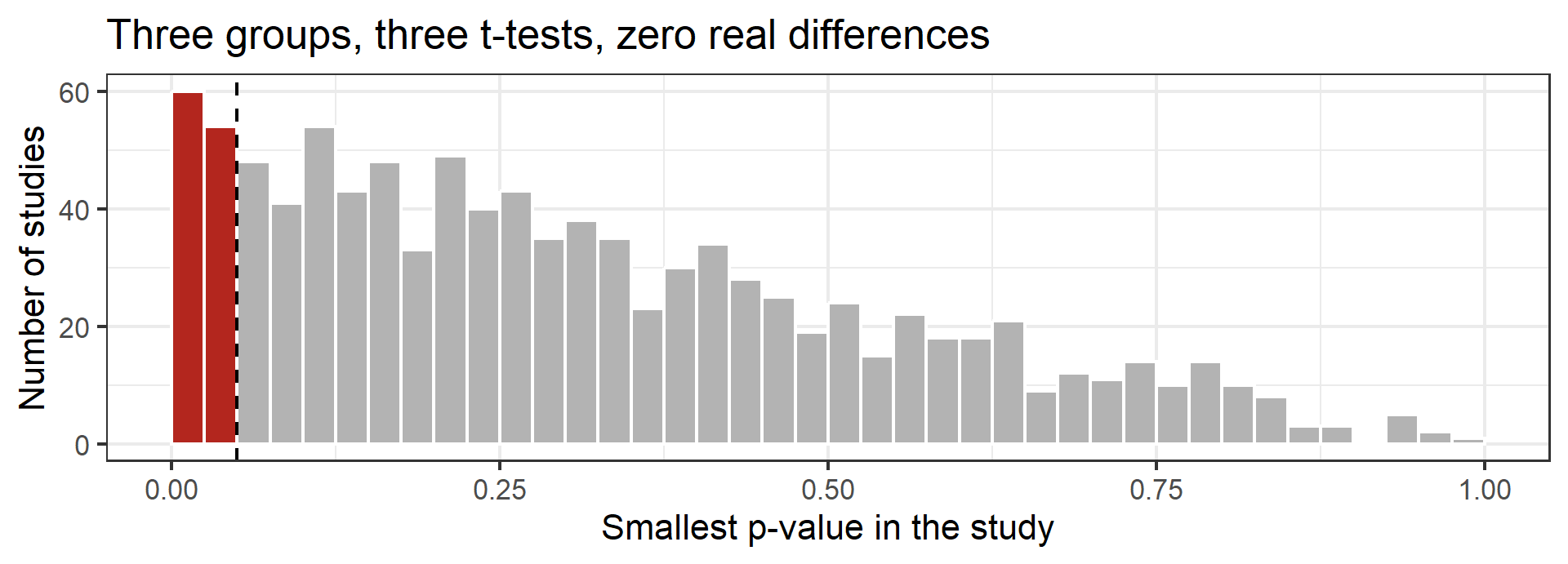
Three groups drawn from the same population, every pairwise t-test run, repeated 1,000 times. About 12% of these studies produced at least one “significant” difference. None were real.
It gets worse fast
| Groups | Pairwise tests | False-positive rate |
|---|---|---|
| 2 | 1 | 4.9% ← as advertised |
| 3 | 3 | 12.3% |
| 4 | 6 | 20.2% |
| 5 | 10 | 29.2% |
20,000 simulated studies per row, n = 30 per group, all groups from the same population.
- The naive formula (\(1-.95^{10}\) = 40% for five groups) overstates it, because the tests overlap
- But the honest number is still six times the rate you think you are running
Note
JAMOVI has no built-in simulator, so this one is a demo rather than something to click along with. The code is on the R slides, and the activity has a version you can run if you are curious.
This is why we start with one omnibus test, and why pairwise comparisons get corrected.
Two groups needed one dummy. Three need two.
| Group | Junior+ |
Sophomore |
|---|---|---|
| First year (reference) | 0 | 0 |
| Junior+ | 1 | 0 |
| Sophomore | 0 | 1 |
- \(k\) groups → \(k - 1\) dummy variables
- Every group gets a unique pattern of 0s and 1s
- The reference group is the one that is all zeros
JAMOVI builds these the moment you drop a nominal variable into Factors.
The model
Analyses → Regression → Linear Regression
Dependent:
hours_of_sleep· Factors:year_groupModel Fit: tick R² and Overall Model Test (F test)
Model Fit
| R² | F | df1 | df2 | p |
|---|---|---|---|---|
| 0.111 | 6.02 | 2 | 96 | 0.003 |
Model Coefficients
| Predictor | Estimate | SE | t | p |
|---|---|---|---|---|
| Intercept | 6.13 | 0.159 | 38.5 | < .001 |
| Junior+ – First year | 0.79 | 0.228 | 3.47 | < .001 |
| Sophomore – First year | 0.35 | 0.261 | 1.34 | 0.184 |
Reading it
\[\widehat{sleep} = 6.13 + 0.79(junior^+) + 0.35(sophomore)\]
- Intercept 6.13 = mean sleep of first-years (the reference)
- +0.79 = juniors+ sleep 0.79 hours more than first-years
- +0.35 = sophomores sleep 0.35 hours more than first-years, and that one is not significant
- Every estimate is a comparison to the reference group — not to each other
So where is sophomore vs junior+? It isn’t in this table. JAMOVI even names the rows that way: Junior+ – First year.
The omnibus F test
F(2, 96) = 6.02, p = .003, R² = .111
- \(H_0\): all three population means are equal
- A small p says at least one group differs — it does not say which
- This is the ANOVA you already know. Same model, different summary.
Run it the classic way and compare:
Analyses → ANOVA → ANOVA · Dependent
hours_of_sleep, Fixed Factoryear_groupTick η² under Effect Size
Same F. Same p. η² = .111 — the same number as R².
Getting the comparison the table hid
ANOVA → Post Hoc Tests
Move
year_groupacross · Correction: Tukey
| Comparison | Mean difference | ptukey |
|---|---|---|
| First year − Junior+ | −0.79 | 0.002 |
| First year − Sophomore | −0.35 | 0.377 |
| Junior+ − Sophomore | 0.44 | 0.222 |
- The omnibus test was significant because of one of the three comparisons
- Without the pairwise step you would not know which
Marginal means
ANOVA → Estimated Marginal Means
Add year_group to a term box and tick Marginal means plots and Marginal means tables.
With one factor these are just the group means — but the plot (with error bars) is the figure you want in a talk, and in Week 9 these become the only sane way to read an interaction.
Writing it up
Average nightly sleep differed significantly across year in school, F(2, 96) = 6.02, p = .003, \(\eta^2\) = .11. First-year students reported the least sleep (M = 6.13, SD = 1.28), followed by sophomores (M = 6.48, SD = 0.90) and juniors or above (M = 6.92, SD = 0.64). Tukey-adjusted comparisons indicated that juniors and above slept significantly more than first-year students, p = .002; no other pairwise comparison was significant.
Tip
Notice the shape: omnibus test → group descriptives → which pairs differ. In that order, every time.
JAMOVI’s tables are nearly APA already — right-click → Export to drop them into Word.
And the obvious caveat
Nobody was randomly assigned to be a first-year.
- Maybe upper-year students have more control over their schedules
- Maybe the heavy-sleep-deprivation majors drop out before junior year
- Maybe first-years live in noisier housing
The model is fine. The causal claim is not available — same lesson as Lab 6. Next week’s lab is the exception that proves the rule: a study where people were randomly assigned.
What the model assumes
- Independence — one row per student, no nesting (Week 13 relaxes this)
- Normality of the residuals — not of the raw scores
- Equal variances across groups (homogeneity) — remember SD = 1.28 vs 0.64
ANOVA → Assumption Checks
Homogeneity test (Levene’s) · Normality test (Shapiro-Wilk) · Q-Q plot
If homogeneity fails, JAMOVI offers Welch’s correction right in the One-Way ANOVA panel.
The big picture so far
| What you want | Where it lives in JAMOVI | What people call it |
|---|---|---|
| Continuous predictor | Regression → Linear Regression (Covariates) | Regression |
| 2 groups | T-Tests, or Linear Regression (Factors) | t-test |
| 3+ groups | ANOVA, or Linear Regression (Factors) | One-way ANOVA |
| Several predictors | Covariates and Factors together | Multiple regression (Week 8) |
One machine. You are just changing what goes in the boxes.
JAMOVI ↔︎ R cheat sheet
| What you want | JAMOVI | R |
|---|---|---|
| Group descriptives | Descriptives → Split by | group_by() %>% summarize() |
| Two-group test | T-Tests → Independent Samples | t.test(y ~ g, var.equal = TRUE) |
| Groups as a line | Linear Regression → Factors | lm(y ~ g) |
| Omnibus F | Model Fit → Overall Model Test | anova(mod) / summary(aov()) |
| Change reference group | Reference Levels | relevel() / fct_relevel() |
| Pairwise comparisons | ANOVA → Post Hoc (Tukey) | emmeans(mod, pairwise ~ g) |
| Effect size | Cohen’s d box · η² box | effectsize::cohens_d() · glance()$r.squared |
| Group means plot | Estimated Marginal Means | emmeans() + plot() |
| Make a grouping variable | Data → Compute → IF(...) |
mutate(case_when(...)) |
🛠️ Activity Stop 2: Parts B & C
Tip
Same Question, Three Ways · ~30 min · Pairs
Part B: three Pokémon types, from descriptives to a written-up result
Part C: choose a reference group on purpose, and see what changes (and what doesn’t)
For next time
📋 Lab 7 — Does the Therapy Work?, due Tuesday 10/6 at 11:59pm
- A real three-arm randomized trial: Individual CBT, Group CBT, Waitlist
- You fit the model, pick the reference group, and write the results
- Five participants dropped out — you will have to decide what to say about that
📖 Chapter 8 — ROS · Chapters 5 & 14.5 — ST · Chapter 15.4 — LSR
Note
Heads up: the midterm project is handed out in two weeks (10/15) and due 10/27. Lab 8 is due Tue 10/13, which is during Fall Break — submit it online as usual.