Week 07: Variability & Model Fit

Date: October 8, 2026

Today…

How good is this model, actually?

• Where the variance goes: \(SS_{total} = SS_{model} + SS_{residual}\)
• R², one more time — and what it is not
• The residual standard error: your typical miss, in real units
• The F test as a ratio
• Why R² can only go up, and what to use instead
• 👀 A sneak peek at two predictors

library(here)
library(tidyverse)
library(rio)
library(broom)
library(psych)

options(scipen = 999)

asap <- import(here("files", "data", "asap_data.csv"))

Our data: the ASAP study 😴

400 adolescents, measured on sleep, stress, and mood.

asap %>%
  select(T1_SleepDur, T1_PeerStress, T1_AcadStress, T1_Dep) %>%
  describe(fast = TRUE)

              vars   n mean   sd median   min   max range  skew kurtosis   se
T1_SleepDur      1 400 9.44 1.00   9.41  6.45 12.35  5.90  0.16    -0.25 0.05
T1_PeerStress    2 400 7.93 1.77   7.89  2.86 13.34 10.48  0.23     0.21 0.09
T1_AcadStress    3 400 5.02 1.83   4.97 -0.35 10.63 10.98  0.07    -0.12 0.09
T1_Dep           4 400 9.84 2.15  10.05  1.08 15.29 14.21 -0.35     0.25 0.11

Research question: Does how long adolescents sleep predict depressive symptoms?

Part 1: Where Does the Variance Go?

Start with the dumbest possible model

Suppose you had no predictor at all. What is your best guess for anyone’s depression score?

The mean. That’s it. That’s the model.

mean(asap$T1_Dep)

[1] 9.8442

How wrong is that model? Add up every squared miss:

\[SS_{total} = \sum(Y_i - \bar{Y})^2 = 1840.5\]

This is the total variability we are trying to account for. Everything from here is about shrinking it.

Now add a predictor

fit_sleep <- lm(T1_Dep ~ T1_SleepDur, data = asap)
tidy(fit_sleep)

# A tibble: 2 × 5
  term        estimate std.error statistic   p.value
  <chr>          <dbl>     <dbl>     <dbl>     <dbl>
1 (Intercept)   15.0       0.985     15.3  1.000e-41
2 T1_SleepDur   -0.549     0.104     -5.30 1.96 e- 7

Each additional hour of sleep is associated with 0.55 fewer points of depression.

But our question today is different: how much better is this line than the mean?

Three distances, one observation

For any single adolescent:

\[\underbrace{Y_i - \bar{Y}}_{\text{total}} = \underbrace{\hat{Y_i} - \bar{Y}}_{\text{model}} + \underbrace{Y_i - \hat{Y_i}}_{\text{residual}}\]

• Total: how far this person is from the overall mean
• Model: how far the line moved them from the mean
• Residual: how far the line still missed

Square them, add them up across all 400 people, and the same decomposition holds:

\[SS_{total} = SS_{model} + SS_{residual}\]

See it in the numbers

anova(fit_sleep)

Analysis of Variance Table

Response: T1_Dep
             Df  Sum Sq Mean Sq F value       Pr(>F)    
T1_SleepDur   1  121.16  121.16  28.045 0.0000001965 ***
Residuals   398 1719.39    4.32                         
---
Signif. codes:  0 '***' 0.001 '**' 0.01 '*' 0.05 '.' 0.1 ' ' 1

• \(SS_{model}\) = 121.2 — variability the line accounts for
• \(SS_{residual}\) = 1719.4 — variability it does not
• Together: 121.2 + 1719.4 = 1840.5 = \(SS_{total}\) ✅

R² is just a share

\[R^2 = \frac{SS_{model}}{SS_{total}} = \frac{121.2}{1840.5} = .066\]

glance(fit_sleep) %>% select(r.squared, adj.r.squared, sigma, statistic, p.value)

# A tibble: 1 × 5
  r.squared adj.r.squared sigma statistic     p.value
      <dbl>         <dbl> <dbl>     <dbl>       <dbl>
1    0.0658        0.0635  2.08      28.0 0.000000196

6.6% of the variability in depression is accounted for by sleep duration.

Which means 93.4% is not. Both halves of that sentence are the finding.

Small R², strong evidence

R² = .066

Sleep duration tells us very little about any individual adolescent’s depression.

p < .001

With n = 400, we are confident the slope is not zero.

Important

These are answers to different questions. “Is there an effect?” and “how much does it explain?” are not the same, and a p-value only answers the first.

This is normal in psychology. Behavior has many causes; one predictor rarely owns much of the variance.

Part 2: Fit in Real Units

R² is unitless. That’s a problem.

“.066” does not tell you whether this model is useful for a clinician.

The residual standard error does. It is roughly the size of a typical miss, in the units of the outcome:

\[RSE = \sqrt{\frac{SS_{residual}}{n - k - 1}} = \sqrt{\frac{1719.4}{398}} = 2.08\]

glance(fit_sleep)$sigma

[1] 2.078476

sd(asap$T1_Dep)

[1] 2.147764

The comparison that matters

• Guess the mean for everyone → you are off by about 2.15 points on average
• Use the model → you are off by about 2.08 points

We bought ourselves about 0.07 points of accuracy.

Tip

That is the honest way to describe a small R² to a non-statistician: not “6.6% of variance,” which means nothing to most people, but “knowing how long a teenager slept barely improves our guess about their mood.”

The F test is a ratio

\[F = \frac{MS_{model}}{MS_{residual}} = \frac{\text{variance the model explains, per predictor}}{\text{variance it doesn't, per leftover df}}\]

glance(fit_sleep) %>% select(statistic, df, df.residual, p.value)

# A tibble: 1 × 4
  statistic    df df.residual     p.value
      <dbl> <dbl>       <int>       <dbl>
1      28.0     1         398 0.000000196

• \(F\) = 28.05 on 1 and 398 df
• If the model explained nothing, F would hover around 1
• With one predictor, \(F = t^2\): \((-5.30)^2 = 28.05\) ✅ — the same test again

Part 3: Adding Predictors 👀

Does peer stress help?

fit_two <- lm(T1_Dep ~ T1_SleepDur + T1_PeerStress, data = asap)
tidy(fit_two)

# A tibble: 3 × 5
  term          estimate std.error statistic  p.value
  <chr>            <dbl>     <dbl>     <dbl>    <dbl>
1 (Intercept)     13.0      1.14       11.5  1.74e-26
2 T1_SleepDur     -0.504    0.103      -4.89 1.47e- 6
3 T1_PeerStress    0.201    0.0585      3.43 6.57e- 4

Both predictors are significant. The sleep slope barely moved (−0.55 → −0.50).

What happened to fit?

Model	R²	Adjusted R²	RSE
Sleep only	.066	.064	2.078
Sleep + peer stress	.093	.088	2.051

• \(\Delta R^2\) = .027 — peer stress accounts for 2.7% beyond sleep
• The typical miss dropped from 2.078 to 2.051
• Both numbers point the same way: a modest improvement

Now let’s add something useless

fit_three <- lm(T1_Dep ~ T1_SleepDur + T1_PeerStress + T1_AcadStress, data = asap)
tidy(fit_three)

# A tibble: 4 × 5
  term          estimate std.error statistic  p.value
  <chr>            <dbl>     <dbl>     <dbl>    <dbl>
1 (Intercept)   13.0        1.14      11.4   3.29e-26
2 T1_SleepDur   -0.503      0.104     -4.84  1.83e- 6
3 T1_PeerStress  0.202      0.0590     3.42  6.91e- 4
4 T1_AcadStress -0.00703    0.0570    -0.123 9.02e- 1

Academic stress: b = −0.007, p = .90. As close to nothing as you will ever see.

Watch what R² does

Model	R²	Adjusted R²	RSE
Sleep only	.0658	.0635	2.078
+ peer stress	.0928	.0882	2.051
+ academic stress	.0928	.0859 ⬇️	2.053 ⬆️

• R² did not go down — it never can
• Adjusted R² did, and the typical miss got worse

Why R² can only climb

Adding a predictor gives OLS one more knob to turn. At worst it sets the coefficient near zero and fit stays the same; usually it catches a sliver of noise and R² ticks up.

\[R^2_{adj} = 1 - (1 - R^2)\frac{n - 1}{n - k - 1}\]

Every predictor \(k\) costs you something. Adjusted R² only rises if the new variable earns its place.

Important

R² is not a model-selection tool. The biggest R² always belongs to the model with the most predictors. Week 11 gives us honest ways to compare models.

⏱️ One last thing: look at the residuals

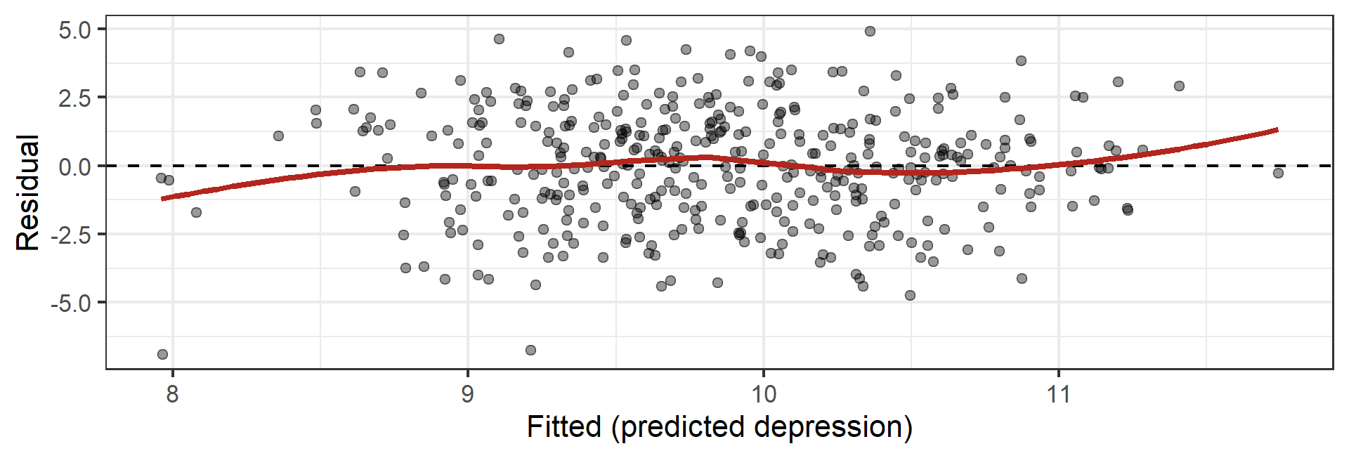
We spent all day computing \(SS_{residual}\). Let’s actually look at the residuals instead of just squaring them.

augment(fit_two) %>% 
  ggplot(aes(x = .fitted, y = .resid)) +
  geom_point(alpha = .4) +
  geom_hline(yintercept = 0, linetype = "dashed") +
  geom_smooth(se = FALSE, color = "#B3261E") +
  labs(x = "Fitted (predicted depression)", y = "Residual") +
  theme_bw(base_size = 16)

A shapeless cloud centered on zero. That is what “nothing obviously wrong” looks like.

What you are glancing for

set.seed(640)
n <- 200
x <- runif(n, 0, 10)

sims <- bind_rows(
  tibble(kind = "1. Healthy",          x = x, y = 2 + 0.8 * x + rnorm(n, 0, 2)),
  tibble(kind = "2. Curve (wrong shape)", x = x, y = 2 + 0.8 * x^2 + rnorm(n, 0, 6)),
  tibble(kind = "3. Funnel (spread grows)", x = x, y = 2 + 0.8 * x + rnorm(n, 0, 0.4 * x)),
  tibble(kind = "4. One strange point",  x = x, y = 2 + 0.8 * x + rnorm(n, 0, 2))
) %>% 
  mutate(y = if_else(kind == "4. One strange point" & row_number() == n(), y + 40, y))

sims %>% 
  group_by(kind) %>% 
  group_modify(~ augment(lm(y ~ x, data = .x))) %>% 
  ggplot(aes(x = .fitted, y = .resid)) +
  geom_point(alpha = .4, size = 1) +
  geom_hline(yintercept = 0, linetype = "dashed") +
  facet_wrap(~ kind, scales = "free") +
  labs(x = "Fitted", y = "Residual") +
  theme_bw(base_size = 13)

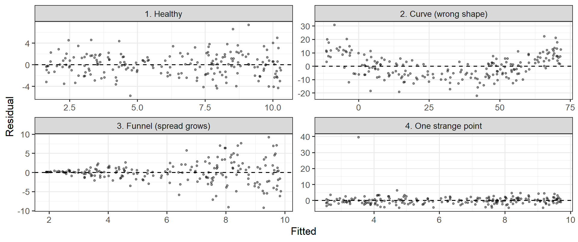
• Curve → the line is the wrong shape for these data
• Funnel → the model is more wrong for some people than others
• Strange point → one observation may be running the whole model (remember the 1,000-books reader?)

Note

That is the entire diagnostic toolkit for now: plot the residuals, look for a pattern. Week 10 turns each of these into a named assumption with a proper test. For the midterm, the glance is enough.

🛠️ Activity: Does the Algorithm Know What a Hit Is?

Tip

Week 7 Exercises · ~45 min · Pairs

Spotify data: 952 popular songs, with danceability, energy, valence, acousticness — and streams.

• Four audio features together explain about 1% of streams
• One boring variable explains 62%
• You will find it, and then explain why the fancy features lost

Open the activity

✍️ Wrap-Up

Finish these at the bottom of your activity file:

1. In one sentence, explain R² to someone who has never taken statistics.
2. Why can a predictor be statistically significant and still barely improve a model?
3. One thing that is still muddy → journal.

For next time

📋 Lab 8 — How Good Is This Model?, due Tuesday 10/13 at 11:59pm

Warning

10/13 is during Fall Break. The lab is submitted online as usual — nothing to hand in physically, and no class that Monday or Tuesday.

• Model fit on a real anxiety dataset, in the units people care about
• Ends with a sneak peek: one predictor that looks useless alone, and what happens when you add a second

📖 Chapter 10 — ROS (for next week’s multiple regression)

📂 Midterm Project — posted today

The Midterm Project is up on the website now. Due Tuesday, 10/27 at 11:59pm. It is worth 200 points (20% of your grade).

• Parts 1-5 use only what you already know - cleaning, scoring, describing, one-predictor models. You can start this weekend.
• Part 6 needs multiple regression, which is next class (10/15).
• You pick your own research question. Read the whole thing before you leave today.

No lab is due in Weeks 9 or 10, so that time is yours for the project.