Week 07: Variability & Model Fit with JAMOVI
Date: October 8, 2026
Today…
How good is this model, actually?
- Where the variance goes: \(SS_{total} = SS_{model} + SS_{residual}\)
- R², one more time — and what it is not
- The typical miss, in real units
- The F test as a ratio
- Why R² can only go up, and what to use instead
- 👀 A sneak peek at two predictors
Note
This is the JAMOVI version. Same data, same numbers as the R deck. JAMOVI is genuinely better than base R at one thing today — comparing nested models — so stick around for Part 3.
Our data: the ASAP study 😴
400 adolescents, measured on sleep, stress, and mood.
☰ Menu → Open → Browse →
asap_data.csv
Analyses → Exploration → Descriptives ·
T1_SleepDur,T1_PeerStress,T1_AcadStress,T1_Dep
| Variable | N | Mean | SD |
|---|---|---|---|
T1_SleepDur (hours) |
400 | 9.45 | 1.00 |
T1_PeerStress |
400 | 7.93 | 1.77 |
T1_AcadStress |
400 | 5.02 | 1.83 |
T1_Dep |
400 | 9.84 | 2.15 |
Research question: Does how long adolescents sleep predict depressive symptoms?
Part 1: Where Does the Variance Go?
Start with the dumbest possible model
Suppose you had no predictor at all. What is your best guess for anyone’s depression score?
The mean: 9.84. That’s it. That’s the model.
How wrong is that model? Add up every squared miss:
\[SS_{total} = \sum(Y_i - \bar{Y})^2 = 1840.5\]
This is the total variability we are trying to account for. Everything from here is about shrinking it.
Now add a predictor
Analyses → Regression → Linear Regression
Dependent Variable:
T1_Dep· Covariates:T1_SleepDurModel Fit: tick R², Adjusted R², RMSE, Overall Model Test
Model Coefficients: tick Omnibus ANOVA Test
| Predictor | Estimate | SE | t | p |
|---|---|---|---|---|
| Intercept | 15.031 | 0.985 | 15.26 | < .001 |
| T1_SleepDur | −0.549 | 0.104 | −5.30 | < .001 |
Each additional hour of sleep is associated with 0.55 fewer points of depression. But today’s question is: how much better is this line than the mean?
Three distances, one observation
For any single adolescent:
\[\underbrace{Y_i - \bar{Y}}_{\text{total}} = \underbrace{\hat{Y_i} - \bar{Y}}_{\text{model}} + \underbrace{Y_i - \hat{Y_i}}_{\text{residual}}\]
- Total: how far this person is from the overall mean
- Model: how far the line moved them from the mean
- Residual: how far the line still missed
Square them, add them up across all 400 people, and the same decomposition holds:
\[SS_{total} = SS_{model} + SS_{residual}\]
See it in the numbers
The Omnibus ANOVA Test table you just ticked:
| Term | Sum of Squares | df | Mean Square | F | p |
|---|---|---|---|---|---|
| T1_SleepDur | 121.2 | 1 | 121.2 | 28.05 | < .001 |
| Residuals | 1719.4 | 398 | 4.32 |
- \(SS_{model}\) = 121.2 — variability the line accounts for
- \(SS_{residual}\) = 1719.4 — variability it does not
- Together: 121.2 + 1719.4 = 1840.5 = \(SS_{total}\) ✅
R² is just a share
\[R^2 = \frac{SS_{model}}{SS_{total}} = \frac{121.2}{1840.5} = .066\]
Model Fit Measures
| R | R² | Adjusted R² | RMSE |
|---|---|---|---|
| 0.257 | 0.0658 | 0.0635 | 2.073 |
6.6% of the variability in depression is accounted for by sleep duration.
Which means 93.4% is not. Both halves of that sentence are the finding.
Small R², strong evidence
R² = .066
Sleep duration tells us very little about any individual adolescent’s depression.
p < .001
With n = 400, we are confident the slope is not zero.
Important
These are answers to different questions. “Is there an effect?” and “how much does it explain?” are not the same, and a p-value only answers the first.
This is normal in psychology. Behavior has many causes; one predictor rarely owns much of the variance.
Part 2: Fit in Real Units
R² is unitless. That’s a problem.
“.066” does not tell you whether this model is useful for a clinician.
RMSE does. It is roughly the size of a typical miss, in the units of the outcome:
\[RMSE \approx \sqrt{\frac{SS_{residual}}{n}} = \sqrt{\frac{1719.4}{400}} = 2.07\]
Note
JAMOVI’s RMSE divides by n; R’s “residual standard error” divides by the degrees of freedom (2.08 here). Same idea, trivially different arithmetic — don’t let the two labels confuse you.
The comparison that matters
- Guess the mean for everyone → you are off by about 2.15 points on average
- Use the model → you are off by about 2.07 points
We bought ourselves about 0.08 points of accuracy.
Tip
That is the honest way to describe a small R² to a non-statistician: not “6.6% of variance,” which means nothing to most people, but “knowing how long a teenager slept barely improves our guess about their mood.”
The F test is a ratio
\[F = \frac{MS_{model}}{MS_{residual}} = \frac{121.2}{4.32} = 28.05\]
Overall Model Test
| F | df1 | df2 | p |
|---|---|---|---|
| 28.05 | 1 | 398 | < .001 |
- If the model explained nothing, F would hover around 1
- With one predictor, \(F = t^2\): \((-5.30)^2 = 28.05\) ✅ — the same test again
Part 3: Adding Predictors 👀
JAMOVI’s best trick: Model Builder
Linear Regression → Model Builder
Block 1:
T1_SleepDurClick + Add New Block → Block 2:
T1_PeerStress
Now tick Model Comparisons under Model Fit.
JAMOVI will fit both models and test the difference between them — which is exactly the question “did peer stress earn its place?”
Does peer stress help?
Model Comparisons
| Comparison | ΔR² | F | df1 | df2 | p |
|---|---|---|---|---|---|
| Model 1 − Model 2 | 0.027 | 11.78 | 1 | 397 | < .001 |
Model Fit Measures
| Model | R² | Adjusted R² | RMSE |
|---|---|---|---|
| 1. Sleep only | .0658 | .0635 | 2.073 |
| 2. + peer stress | .0928 | .0882 | 2.043 |
- \(\Delta R^2\) = .027 — peer stress accounts for 2.7% beyond sleep
- The typical miss dropped from 2.073 to 2.043
Now let’s add something useless
+ Add New Block → Block 3:
T1_AcadStress
| Predictor | Estimate | SE | t | p |
|---|---|---|---|---|
| T1_AcadStress | −0.007 | 0.057 | −0.12 | 0.902 |
Academic stress is as close to nothing as you will ever see.
Watch what R² does
| Model | R² | Adjusted R² | RMSE |
|---|---|---|---|
| 1. Sleep only | .0658 | .0635 | 2.073 |
| 2. + peer stress | .0928 | .0882 | 2.043 |
| 3. + academic stress | .0928 | .0859 ⬇️ | 2.043 |
- R² did not go down — it never can
- Adjusted R² did
- And Model Comparisons reports the block as non-significant, p = .90
Why R² can only climb
Adding a predictor gives the model one more knob to turn. At worst the coefficient sits near zero and fit stays the same; usually it catches a sliver of noise and R² ticks up.
\[R^2_{adj} = 1 - (1 - R^2)\frac{n - 1}{n - k - 1}\]
Every predictor \(k\) costs you something. Adjusted R² only rises if the new variable earns its place.
Important
R² is not a model-selection tool. The biggest R² always belongs to the model with the most predictors. Week 11 gives us honest ways to compare models — and JAMOVI’s Model Comparisons table is the first one.
JAMOVI ↔︎ R cheat sheet
| What you want | JAMOVI | R |
|---|---|---|
| R², adjusted R² | Model Fit Measures | glance(fit) |
| Typical miss | Model Fit → RMSE | glance(fit)$sigma |
| Sums of squares | Model Coefficients → Omnibus ANOVA Test | anova(fit) |
| Overall F | Model Fit → Overall Model Test | glance(fit)$statistic |
| Compare nested models | Model Builder blocks + Model Comparisons | anova(fit1, fit2) |
| ΔR² | Model Comparisons table | subtract two glance() rows |
⏱️ One last thing: look at the residuals
We spent all day computing \(SS_{residual}\). Let’s actually look at the residuals instead of just squaring them.
Linear Regression → Assumption Checks
Tick Residual plots
JAMOVI gives you residuals against fitted values (plus a Q-Q plot). For the ASAP model it is a shapeless cloud centered on zero — which is what “nothing obviously wrong” looks like.
What you are glancing for
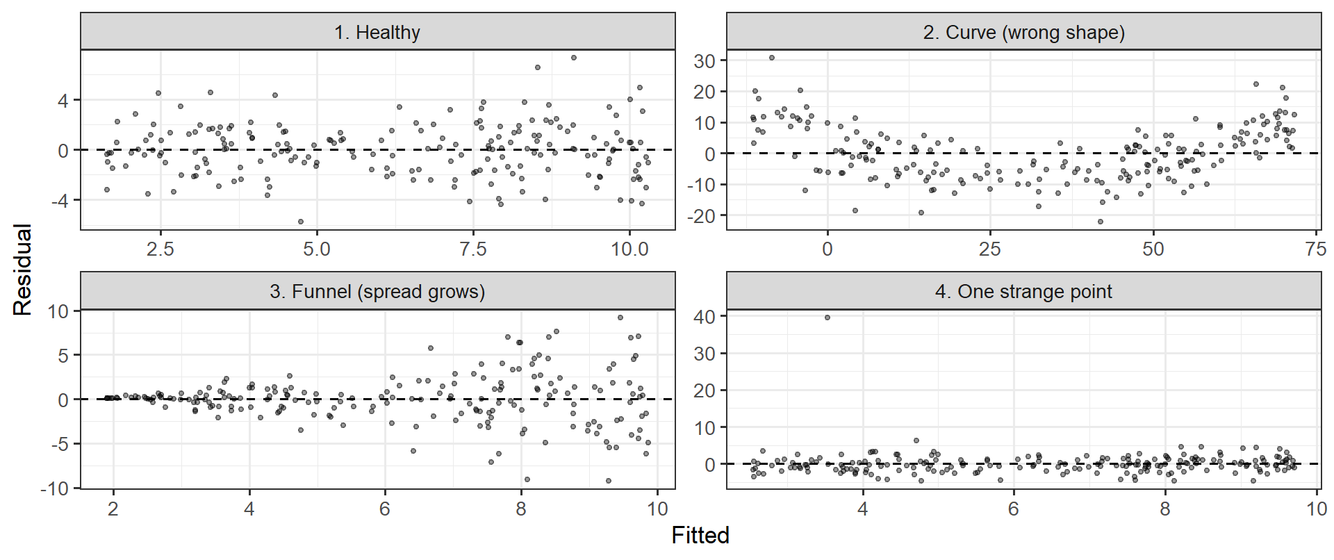
- Curve → the line is the wrong shape for these data
- Funnel → the model is more wrong for some people than others
- Strange point → one observation may be running the whole model (remember the 1,000-books reader?)
Note
That is the entire diagnostic toolkit for now: tick the box, look for a pattern. Week 10 turns each of these into a named assumption with a proper test. For the midterm, the glance is enough.
🛠️ Activity: Does the Algorithm Know What a Hit Is?
Tip
Week 7 Exercises · ~45 min · Pairs
Spotify data: 952 popular songs, with danceability, energy, valence, acousticness — and streams.
- Four audio features together explain about 1% of streams
- One boring variable explains 62%
- You will find it, and then explain why the fancy features lost
✍️ Wrap-Up
Finish these at the bottom of your activity file:
- In one sentence, explain R² to someone who has never taken statistics.
- Why can a predictor be statistically significant and still barely improve a model?
- One thing that is still muddy → journal.
For next time
📋 Lab 8 — How Good Is This Model?, due Tuesday 10/13 at 11:59pm
Warning
10/13 is during Fall Break. The lab is submitted online as usual — nothing to hand in physically, and no class that Monday or Tuesday.
- Model fit on a real anxiety dataset, in the units people care about
- Ends with a sneak peek: one predictor that looks useless alone, and what happens when you add a second
📖 Chapter 10 — ROS (for next week’s multiple regression)
📂 Midterm Project — posted today
The Midterm Project is up on the website now. Due Tuesday, 10/27 at 11:59pm. It is worth 200 points (20% of your grade).
- Parts 1-5 use only what you already know - cleaning, scoring, describing, one-predictor models. You can start this weekend.
- Part 6 needs multiple regression, which is next class (10/15).
- You pick your own research question. Read the whole thing before you leave today.
No lab is due in Weeks 9 or 10, so that time is yours for the project.