Week 09: Multiple Regression II

Date: October 22, 2026

Today…

Groups meet predictors.

A group and a continuous predictor in the same model
Two lines, same slope: what “controlling for” looks like on a plot
What if the slope is different for each group? (interactions)
Simple slopes: the only honest way to report one
Why centering suddenly matters
An interaction that isn’t there — and what to do about it

library(here)
library(tidyverse)
library(rio)
library(broom)
library(easystats)
library(patchwork)

options(scipen = 999)

Two threads, now braided

Week 6

A group is a predictor. Dummy-code it, and the intercept is the reference group’s mean.

Week 8

Put two predictors in one model and each coefficient becomes a holding-constant comparison.

This week: a model with both kinds of predictor in it, and then the question neither week could ask —

Is the slope the same for every group?

Part 1: Group + Continuous

20 students, two things we know about them 🎓

Daily study hours, final grade (on a 10-point scale), and whether the student worked with a tutor.

tutor <- import(here("files", "data", "tutor.csv")) %>%
  mutate(tutor_f = factor(tutor, levels = c(0, 1),
                          labels = c("No tutor", "Tutor")))

tutor %>%
  group_by(tutor_f) %>%
  summarize(n = n(),
            study_m = mean(study), study_sd = sd(study),
            grade_m = mean(grade), grade_sd = sd(grade)) %>%
  mutate(across(where(is.numeric), ~ round(.x, 3)))

# A tibble: 2 × 6
  tutor_f      n study_m study_sd grade_m grade_sd
  <fct>    <dbl>   <dbl>    <dbl>   <dbl>    <dbl>
1 No tutor    10   0.995    0.563    6.76    1.14 
2 Tutor       10   1.64     0.557    8.89    0.526

Two separate stories

m_study <- lm(grade ~ study, data = tutor)
m_tutor <- lm(grade ~ tutor_f, data = tutor)

tidy(m_study)

# A tibble: 2 × 5
  term        estimate std.error statistic  p.value
  <chr>          <dbl>     <dbl>     <dbl>    <dbl>
1 (Intercept)     5.52     0.450     12.3  3.46e-10
2 study           1.75     0.309      5.66 2.27e- 5

tidy(m_tutor)

# A tibble: 2 × 5
  term         estimate std.error statistic  p.value
  <chr>           <dbl>     <dbl>     <dbl>    <dbl>
1 (Intercept)      6.76     0.280     24.1  3.75e-15
2 tutor_fTutor     2.13     0.397      5.37 4.19e- 5

Study: each extra hour → +1.75 grade points, \(R^2\) = .640
Tutor: tutored students score +2.13 higher, \(R^2\) = .616

Two strong, significant, nearly equally powerful predictors. Should we just add them up?

Look first 👀

Code

tutor %>%
  ggplot(aes(x = study, y = grade, color = tutor_f)) +
  geom_point(size = 3, alpha = .85) +
  labs(x = "Daily study hours", y = "Final grade", color = NULL) +
  theme_bw(base_size = 16)

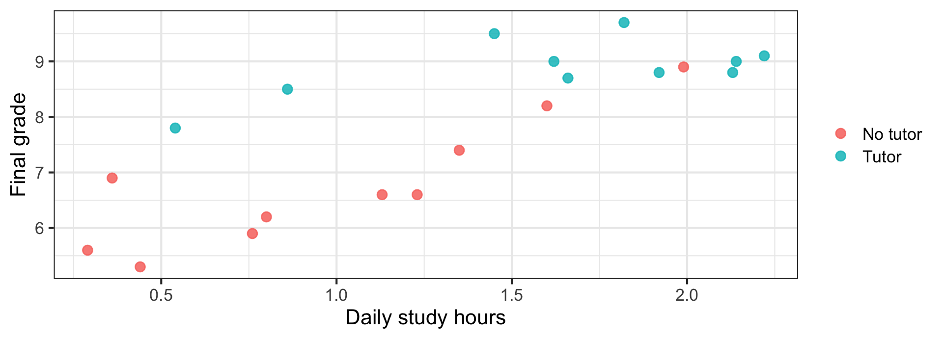
Notice where the tutored students sit on the x-axis. They also study more (1.64 vs 0.99 hours). The two predictors are entangled: r = .52.

Both at once

m_both <- lm(grade ~ study + tutor_f, data = tutor)
summary(m_both)


Call:
lm(formula = grade ~ study + tutor_f, data = tutor)

Residuals:
    Min      1Q  Median      3Q     Max 
-0.8064 -0.4470 -0.2686  0.5413  0.9681 

Coefficients:
             Estimate Std. Error t value         Pr(>|t|)    
(Intercept)    5.5882     0.3198  17.474 0.00000000000269 ***
study          1.1777     0.2565   4.592         0.000259 ***
tutor_fTutor   1.3751     0.3183   4.320         0.000465 ***
---
Signif. codes:  0 '***' 0.001 '**' 0.01 '*' 0.05 '.' 0.1 ' ' 1

Residual standard error: 0.6096 on 17 degrees of freedom
Multiple R-squared:  0.8285,    Adjusted R-squared:  0.8083 
F-statistic: 41.07 on 2 and 17 DF,  p-value: 0.0000003096

glance(m_both) %>% select(r.squared, adj.r.squared, sigma)

# A tibble: 1 × 3
  r.squared adj.r.squared sigma
      <dbl>         <dbl> <dbl>
1     0.829         0.808 0.610

Predictor	Alone	Together	Change
`study`	1.750	1.178	−33%
`tutor_f`	2.130	1.375	−35%

\(R^2\): .640 → .829

Both effects shrank. Both are still real.

Part of “the tutoring effect” was that tutored students study more
Part of “the studying effect” was that heavy studiers were more likely to have a tutor
Hold one still and each one keeps only the part that is its own

Important

Shrinkage is not failure. The bivariate numbers were double-counting shared credit. These are the honest ones — and both survive: p = .0003 and p = .0005.

What the model looks like

\[\widehat{Grade} = 5.588 + 1.178(Study) + 1.375(Tutor)\]

Tutor is 0 or 1, so this is two lines
No tutor: \(\widehat{Grade} = 5.588 + 1.178(Study)\)
Tutor: \(\widehat{Grade} = (5.588 + 1.375) +1.178(Study)\)

Same slope. Different intercept. The model has assumed that tutoring shifts the line up without changing its steepness.

Parallel lines, by construction

Code

tutor %>%
  mutate(fit = predict(m_both)) %>%
  ggplot(aes(x = study, y = grade, color = tutor_f)) +
  geom_point(size = 3, alpha = .6) +
  geom_line(aes(y = fit), linewidth = 1.2) +
  labs(x = "Daily study hours", y = "Final grade", color = NULL,
       title = "grade ~ study + tutor") +
  theme_bw(base_size = 16)

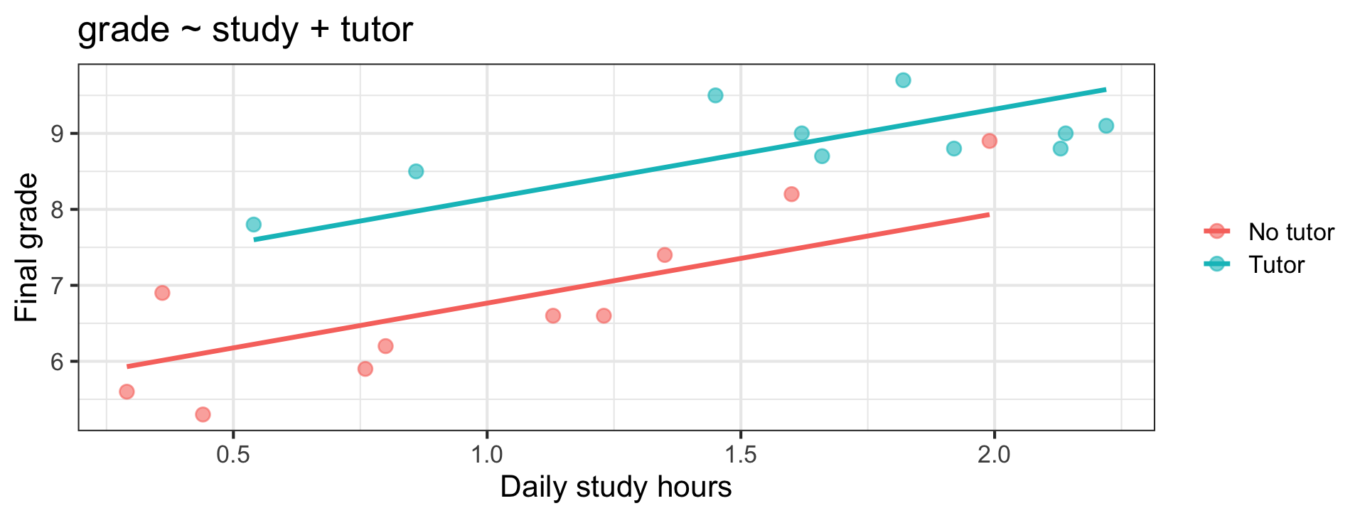
The gap between the lines is 1.375 at every value of study. That is not something we found. It is something we imposed.

Did the group earn its place?

anova(m_study, m_both)

Analysis of Variance Table

Model 1: grade ~ study
Model 2: grade ~ study + tutor_f
  Res.Df     RSS Df Sum of Sq      F   Pr(>F)    
1     18 13.2498                                 
2     17  6.3168  1     6.933 18.658 0.000465 ***
---
Signif. codes:  0 '***' 0.001 '**' 0.01 '*' 0.05 '.' 0.1 ' ' 1

\(\Delta R^2\) = .829 − .640 = .188
\(F\)(1, 17) = 18.66, p = .0005
Typical miss: 0.858 → 0.610 grade points

Tip

This is exactly the midterm’s Part 6 table. One continuous predictor, one categorical predictor, one model with both, and the comparison between them.

💻 Your Turn - Part 1

Open the activity

Part 2: What If The Slopes Differ?

The assumption we never checked

Parallel lines say: tutoring helps every student by the same amount, no matter how much they study.

Is that plausible?

Maybe tutoring mostly helps students who are not putting in hours
Maybe tutoring compounds — it helps most the students who already study
Maybe it really is a constant boost

We can test it. All it takes is one more term.

The interaction term

\[Y = b_0 + b_1X + b_2D + b_3(X \times D) + e\]

m_int <- lm(grade ~ study * tutor_f, data = tutor)
summary(m_int)


Call:
lm(formula = grade ~ study * tutor_f, data = tutor)

Residuals:
    Min      1Q  Median      3Q     Max 
-0.5728 -0.3837 -0.1584  0.1838  1.2555 

Coefficients:
                   Estimate Std. Error t value      Pr(>|t|)    
(Intercept)          5.0121     0.3496  14.337 0.00000000015 ***
study                1.7567     0.3095   5.676 0.00003443132 ***
tutor_fTutor         2.9203     0.6418   4.550      0.000328 ***
study:tutor_fTutor  -1.1713     0.4402  -2.661      0.017093 *  
---
Signif. codes:  0 '***' 0.001 '**' 0.01 '*' 0.05 '.' 0.1 ' ' 1

Residual standard error: 0.5232 on 16 degrees of freedom
Multiple R-squared:  0.8811,    Adjusted R-squared:  0.8588 
F-statistic: 39.53 on 3 and 16 DF,  p-value: 0.0000001259

study * tutor_f in R expands to study + tutor_f + study:tutor_f. Never fit the product without both main effects.

The interaction term

sjPlot::tab_model(m_both, m_int)

	grade			grade
Predictors	Estimates	CI	p	Estimates	CI	p
(Intercept)	5.59	4.91 – 6.26	<0.001	5.01	4.27 – 5.75	<0.001
study	1.18	0.64 – 1.72	<0.001	1.76	1.10 – 2.41	<0.001
tutor f [Tutor]	1.38	0.70 – 2.05	<0.001	2.92	1.56 – 4.28	<0.001
study × tutor f [Tutor]				-1.17	-2.10 – -0.24	0.017
Observations	20			20
R² / R² adjusted	0.829 / 0.808			0.881 / 0.859

Reading the interaction

Term	b	p	What it is
intercept	\(b_0\) 5.012	< .001	grade for no tutor, study = 0
`study`	\(b_1\) 1.757	< .001	slope for the reference group (no tutor)
`tutor_f`	\(b_2\) 2.920	.0003	group gap at study = 0 (intercept difference)
`study:tutor_f`	\(b_3\) −1.171	.017	how much the slope changes for tutored students

Important

Once there is an interaction in the model, study is no longer “the” effect of studying. It is the effect of studying for the group coded 0.

Simple slopes

No tutor

\(b_1 = 1.757\)

Each extra hour → +1.76 points

Tutor

\(b_1 + b_3 = 1.757 - 1.171\)

Each extra hour → +0.59 points

coef(m_int)[["study"]]

[1] 1.756707

coef(m_int)[["study"]] + coef(m_int)[["study:tutor_fTutor"]]

[1] 0.5853662

Three times steeper without a tutor. Report simple slopes — the raw coefficients mean almost nothing on their own.

Simple Slopes `modelbased`

https://easystats.github.io/modelbased/articles/introduction_comparisons_3.html

estimate_slopes(m_int, "study", by = "tutor_f")

Estimated Marginal Effects

tutor_f  | Slope |   SE |        95% CI | t(16) |      p
--------------------------------------------------------
No tutor |  1.76 | 0.31 | [ 1.10, 2.41] |  5.68 | < .001
Tutor    |  0.59 | 0.31 | [-0.08, 1.25] |  1.87 |  0.080

Marginal effects estimated for study
Type of slope was dY/dX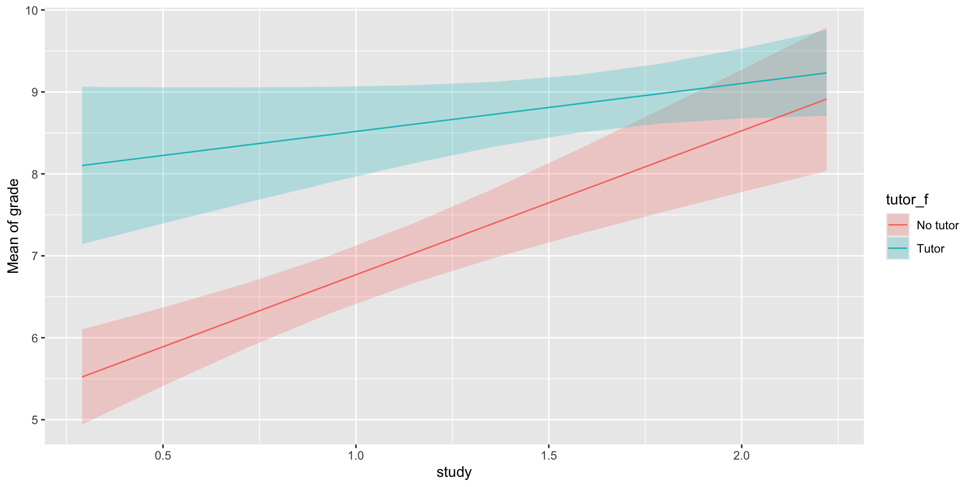

plot(estimate_means(m_int, c("study", "tutor_f")))

Now the picture makes sense

Code

tutor %>%
  ggplot(aes(x = study, y = grade, color = tutor_f)) +
  geom_point(size = 3, alpha = .6) +
  geom_smooth(method = "lm", se = FALSE, linewidth = 1.2) +
  labs(x = "Daily study hours", y = "Final grade", color = NULL,
       title = "grade ~ study * tutor") +
  theme_bw(base_size = 16)

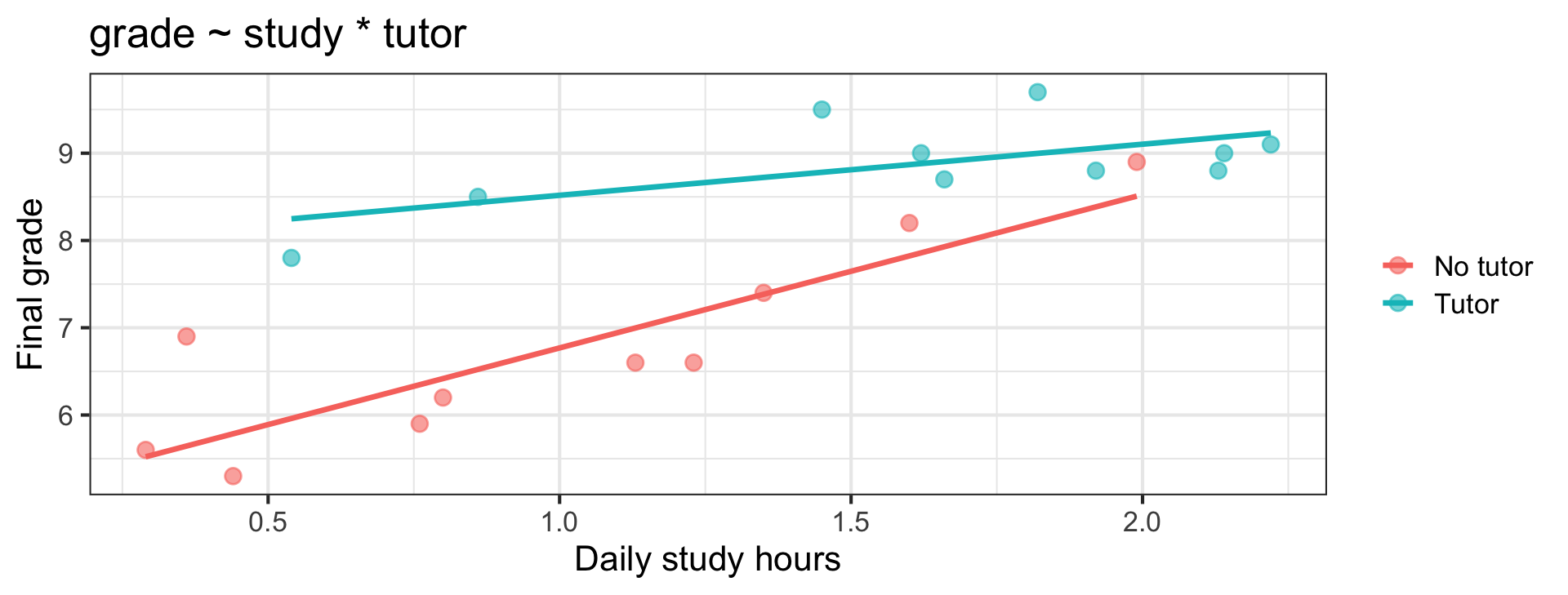
The lines converge. Tutoring buys a lot for a student studying half an hour a day, and nearly nothing for one studying two hours.

https://interactions.jacob-long.com/

Say it in words

An interaction is always symmetric. Both of these are the same finding:

The benefit of tutoring depends on how much a student studies
The payoff of studying depends on whether a student has a tutor

Tip

Pick the direction that answers your research question, say it in one sentence, then show the plot. A reader will believe the plot before they believe the coefficient.

Did the interaction earn its place?

anova(m_both, m_int)

Analysis of Variance Table

Model 1: grade ~ study + tutor_f
Model 2: grade ~ study * tutor_f
  Res.Df    RSS Df Sum of Sq      F  Pr(>F)  
1     17 6.3168                              
2     16 4.3792  1    1.9376 7.0791 0.01709 *
---
Signif. codes:  0 '***' 0.001 '**' 0.01 '*' 0.05 '.' 0.1 ' ' 1

Model	\(R^2\)	adj. \(R^2\)	RSE
additive	.8285	.8083	0.610
+ interaction	.8811	.8588	0.523

\(\Delta R^2\) = .053, \(F\)(1, 16) = 7.08, p = .017. Adjusted \(R^2\) rose. Keep it.

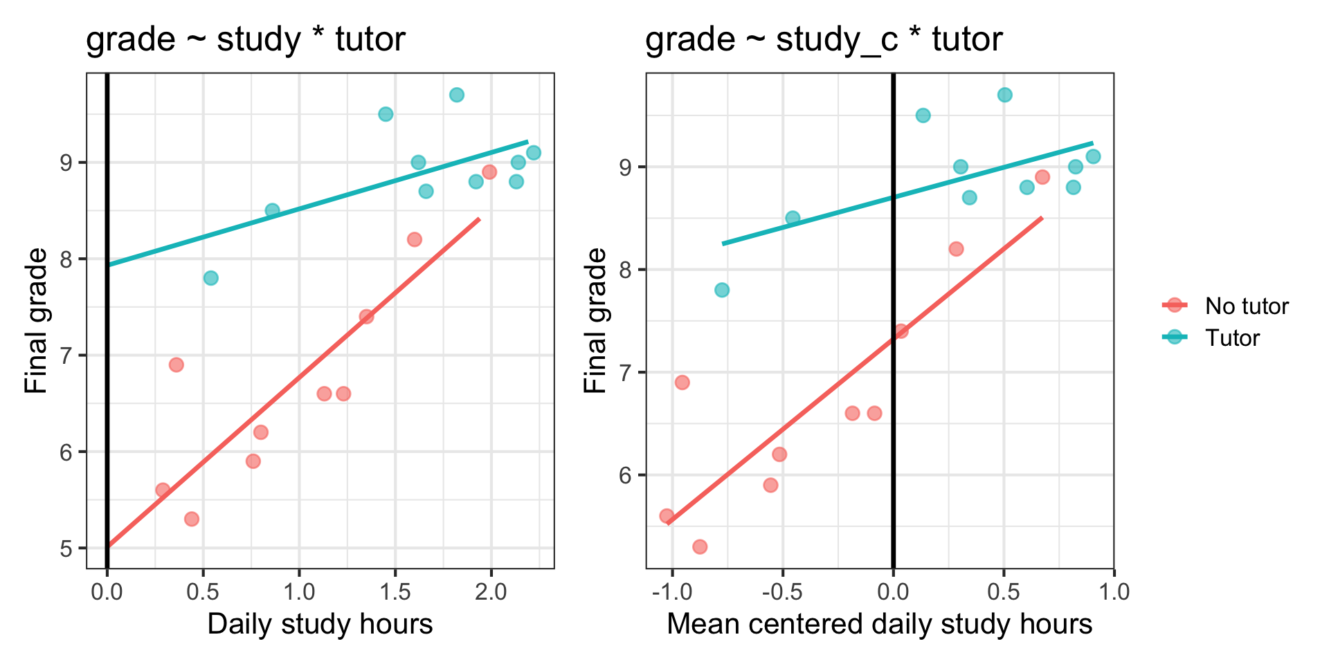
⚠️ Centering is no longer optional

In the interaction model, tutor_f = 2.92 was the group gap at study = 0 — a student who studies zero hours a day. This doesn’t exist. It is purely extrapolation.

tutor_c <- tutor %>% mutate(study_c = study - mean(study))
lm(grade ~ study_c * tutor_f, data = tutor_c) %>% tidy()

# A tibble: 4 × 5
  term                 estimate std.error statistic  p.value
  <chr>                   <dbl>     <dbl>     <dbl>    <dbl>
1 (Intercept)              7.32     0.193     38.0  4.17e-17
2 study_c                  1.76     0.310      5.68 3.44e- 5
3 tutor_fTutor             1.38     0.273      5.05 1.19e- 4
4 study_c:tutor_fTutor    -1.17     0.440     -2.66 1.71e- 2

Mean study = 1.316 hours
Group gap at the mean: 1.379, not 2.92
study_c slope and the interaction: identical — centering did not change the model, only where we read it

Why that matters

Important

Centering a predictor moves the intercept and the other variable’s main effect to a meaningful place. It does not change the interaction, the fit, or the p-value for the interaction.

In a model with an interaction, always center your continuous predictor — or be ready to explain what X = 0 means.

Part 3: When It Isn’t There

100 children, sleep, and parenting 😴

Anxiety scores for 100 children, with hours of sleep and whether parenting was rated Authoritative or Permissive.

kids <- import(here("files", "data", "child_wellbeing.csv")) %>%
  mutate(ps = factor(parenting_style,
                     levels = c("Authoritative", "Permissive")))

kids %>%
  group_by(ps) %>%
  summarise(n = n(),
            sleep_m = mean(sleep_hours),
            anx_m = mean(anxiety_score), anx_sd = sd(anxiety_score)) %>%
  mutate(across(where(is.numeric), ~ round(.x, 3)))

# A tibble: 2 × 5
  ps                n sleep_m anx_m anx_sd
  <fct>         <dbl>   <dbl> <dbl>  <dbl>
1 Authoritative    47    9.51  14.4   5.42
2 Permissive       53    9.36  30.0   6.46

Build it up

k_sleep <- lm(anxiety_score ~ sleep_hours, data = kids)
k_both  <- lm(anxiety_score ~ sleep_hours + ps, data = kids)

tidy(k_sleep)

# A tibble: 2 × 5
  term        estimate std.error statistic  p.value
  <chr>          <dbl>     <dbl>     <dbl>    <dbl>
1 (Intercept)    67.8      7.79       8.70 8.17e-14
2 sleep_hours    -4.78     0.822     -5.82 7.40e- 8

glance(k_sleep)

# A tibble: 1 × 12
  r.squared adj.r.squared sigma statistic      p.value    df logLik   AIC   BIC
      <dbl>         <dbl> <dbl>     <dbl>        <dbl> <dbl>  <dbl> <dbl> <dbl>
1     0.257         0.249  8.50      33.9 0.0000000740     1  -355.  716.  723.
# ℹ 3 more variables: deviance <dbl>, df.residual <int>, nobs <int>

tidy(k_both)

# A tibble: 3 × 5
  term         estimate std.error statistic  p.value
  <chr>           <dbl>     <dbl>     <dbl>    <dbl>
1 (Intercept)     55.0      3.78       14.5 4.09e-26
2 sleep_hours     -4.26     0.393     -10.9 1.92e-18
3 psPermissive    14.9      0.813      18.3 3.33e-33

glance(k_both)

# A tibble: 1 × 12
  r.squared adj.r.squared sigma statistic  p.value    df logLik   AIC   BIC
      <dbl>         <dbl> <dbl>     <dbl>    <dbl> <dbl>  <dbl> <dbl> <dbl>
1     0.833         0.830  4.05      242. 2.02e-38     2  -280.  568.  579.
# ℹ 3 more variables: deviance <dbl>, df.residual <int>, nobs <int>

Sleep alone: −4.78 per hour, \(R^2\) = .257
With parenting: −4.26 per hour; permissive +14.88; \(R^2\) = .833

Note what did not happen

The sleep slope moved from −4.78 to −4.26 — a small shrink.

kids %>%
  group_by(ps) %>%
  summarise(mean_sleep = round(mean(sleep_hours), 3))

# A tibble: 2 × 2
  ps            mean_sleep
  <fct>              <dbl>
1 Authoritative       9.51
2 Permissive          9.36

The two groups sleep almost identically (9.51 vs 9.36 hours). With the predictors nearly unrelated, parenting had almost nothing to take back from sleep — it just explained a huge amount of new variance.

Test the interaction anyway

k_int <- lm(anxiety_score ~ sleep_hours * ps, data = kids)
tidy(k_int)

# A tibble: 4 × 5
  term                     estimate std.error statistic  p.value
  <chr>                       <dbl>     <dbl>     <dbl>    <dbl>
1 (Intercept)                52.9       6.17      8.57  1.71e-13
2 sleep_hours                -4.04      0.645    -6.26  1.08e- 8
3 psPermissive               18.2       7.75      2.35  2.08e- 2
4 sleep_hours:psPermissive   -0.353     0.815    -0.434 6.66e- 1

glance(k_int)

# A tibble: 1 × 12
  r.squared adj.r.squared sigma statistic  p.value    df logLik   AIC   BIC
      <dbl>         <dbl> <dbl>     <dbl>    <dbl> <dbl>  <dbl> <dbl> <dbl>
1     0.833         0.828  4.07      160. 3.24e-37     3  -280.  570.  583.
# ℹ 3 more variables: deviance <dbl>, df.residual <int>, nobs <int>

sleep_hours:psPermissive = −0.353, p = .666.

The fit table tells the story

Model	\(R^2\)	adj. \(R^2\)	RSE
additive	.8330	.8295	4.048
+ interaction	.8333	.8281 ⬇️	4.066 ⬆️

anova(k_both, k_int)

Analysis of Variance Table

Model 1: anxiety_score ~ sleep_hours + ps
Model 2: anxiety_score ~ sleep_hours * ps
  Res.Df    RSS Df Sum of Sq     F Pr(>F)
1     97 1589.8                          
2     96 1586.7  1    3.1077 0.188 0.6655

\(\Delta R^2\) = .0003, \(F\)(1, 96) = 0.19, p = .666. Adjusted \(R^2\) went down.

Parallel lines — this time earned

Code

kids %>%
  ggplot(aes(x = sleep_hours, y = anxiety_score, color = ps)) +
  geom_point(alpha = .6) +
  geom_smooth(method = "lm", se = FALSE, linewidth = 1.2) +
  labs(x = "Sleep (hours)", y = "Anxiety score", color = NULL) +
  theme_bw(base_size = 16)

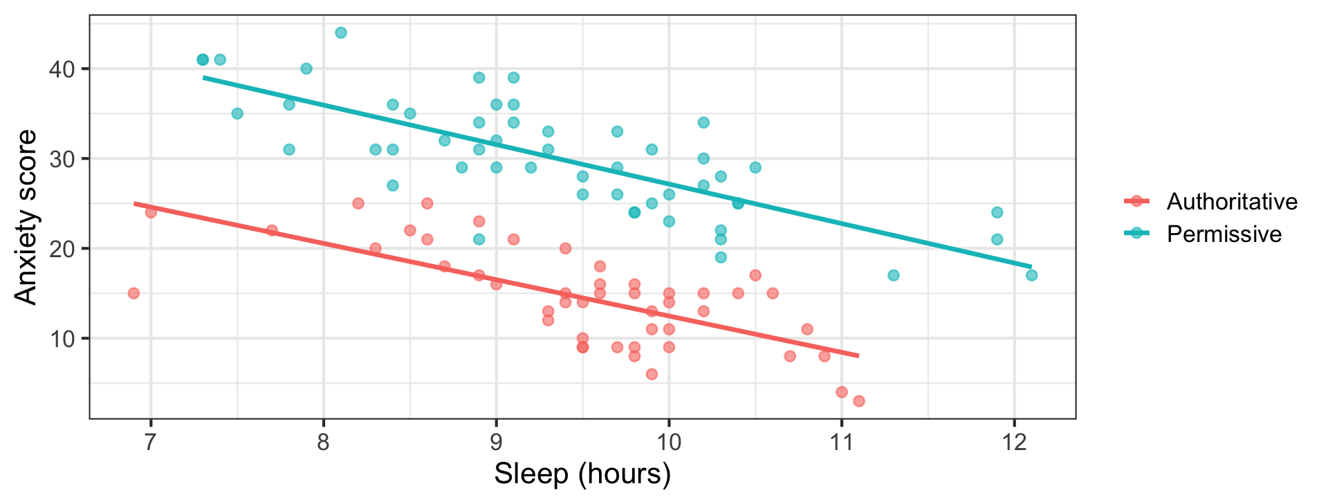
Two lines, essentially the same slope, clearly different heights. Sleep matters the same amount in both groups; the groups just start in different places.

The discipline

Fit the interaction if you have a reason to expect one
Test it
If it is not there, report that and interpret the additive model
Do not keep an interaction you cannot defend just because it was your idea

Warning

A non-significant interaction is not evidence that the slopes are identical — especially with small groups, where you have very little power to detect a difference in slopes. “We found no evidence of moderation” ≠ “there is no moderation.”

The write-up: interaction present

Final grade was regressed on daily study hours (centered), tutoring status, and their interaction (N = 20). The full model accounted for 88.1% of the variance in grades, F(3, 16) = 39.53, p < .001. The interaction was significant, b = −1.17, SE = 0.44, t(16) = −2.66, p = .017, ΔR² = .053. Simple slopes indicated that each additional hour of daily study was associated with a 1.76-point increase in grade for students without a tutor, but only a 0.59-point increase for students with a tutor. At the mean level of study, tutored students scored 1.38 points higher than untutored students (p < .001).

The write-up: interaction absent

Anxiety was regressed on hours of sleep and parenting style (N = 100). The additive model accounted for 83.3% of the variance, F(2, 97) = 241.87, p < .001. Each additional hour of sleep was associated with a 4.26-point decrease in anxiety, holding parenting style constant (p < .001), and children with permissive parenting scored 14.88 points higher than those with authoritative parenting, holding sleep constant (p < .001). A sleep × parenting interaction was tested and was not supported, b = −0.35, p = .666, ΔR² = .0003; the additive model is therefore reported.

Tip

Report that you tested it. A reader who cannot tell whether you looked will assume you looked and did not like the answer.

For next time

📂 Midterm Project — due Tuesday 10/27 at 11:59pm

Five days. If Part 6 is not drafted by this weekend, it will not be good by Tuesday.

You are not required to include an interaction. If you fit one, test it and report the test either way.

📖 Chapter 11 — ROS · Chapter 12.1 — ST (assumptions and diagnostics)

Next week: everything we have been glancing at on residual plots becomes a named assumption with an actual test.

Week 09: Multiple Regression II

Today…

Two threads, now braided

Part 1: Group + Continuous

20 students, two things we know about them 🎓

Two separate stories

Look first 👀

Both at once

Both effects shrank. Both are still real.

What the model looks like

Parallel lines, by construction

Did the group earn its place?

💻 Your Turn - Part 1

Part 2: What If The Slopes Differ?

The assumption we never checked

The interaction term

The interaction term

Reading the interaction

Simple slopes

Simple Slopes modelbased

Now the picture makes sense

Say it in words

Did the interaction earn its place?

⚠️ Centering is no longer optional

Why that matters

Part 3: When It Isn’t There

100 children, sleep, and parenting 😴

Build it up

Note what did not happen

Test the interaction anyway

The fit table tells the story

Parallel lines — this time earned

The discipline

The write-up: interaction present

The write-up: interaction absent

For next time

Simple Slopes `modelbased`