Date: October 29, 2026
Is the model telling the truth?

Is the model telling the truth?
check_model() one panel at a timeIn Week 7 we ended with this:
That is the entire diagnostic toolkit for now: plot the residuals, look for a pattern.
Since then, every model has come with “nothing obviously wrong.” Today each glance gets:
\[ Y_i = b_0 + b_1X_{1i} + b_2X_{2i} + e_i \qquad e_i \sim N(0,\ \sigma) \]
Read that last part out loud: the errors are…
Almost every assumption is a claim about \(e\), the residuals. Very few are about your variables.
Gelman, Hill & Vehtari list the assumptions from most to least important:
Important
The one people test most often (normality) is the one that matters least. The two that matter most (validity, representativeness) cannot be checked with any plot. They are checked by thinking about your design (Week 4).
The most common mistake in a Methods section:
“Shapiro-Wilk tests indicated that anxiety was not normally distributed, so…”
Regression does not assume your predictors or your outcome are normal.
Run diagnostics on the model, not on the raw columns.
| If this fails… | The coefficients (\(b\)) | The SEs, CIs, p-values |
|---|---|---|
| Linearity | Wrong. Wrong-shaped line | Wrong too |
| Independence | Usually fine | Too small. Overconfident |
| Equal variance | Fine | Off. Too big or too small |
| Normality | Fine | Fine in big samples |
| One influential point | Driven by one case | Off |
Two more problems that are not assumptions, but still show up in check_model():
check_model()Week 7: the ASAP study, 400 adolescents. Depression predicted from sleep duration and peer stress.
# A tibble: 3 × 5
term estimate std.error statistic p.value
<chr> <dbl> <dbl> <dbl> <dbl>
1 (Intercept) 13.0 1.14 11.5 1.74e-26
2 T1_SleepDur -0.504 0.103 -4.89 1.47e- 6
3 T1_PeerStress 0.201 0.0585 3.43 6.57e- 4
We interpreted these coefficients three weeks ago. Were we allowed to?
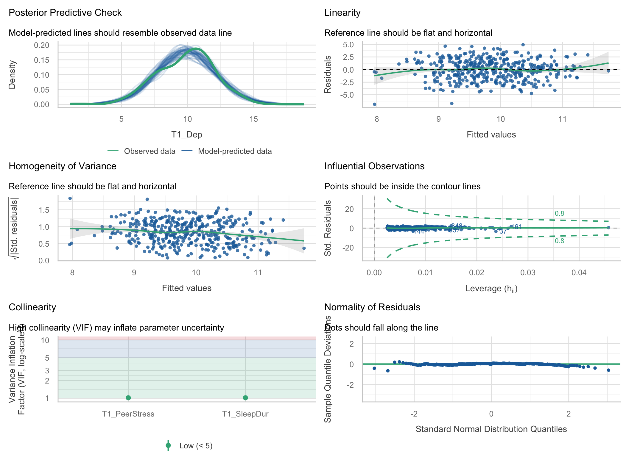
Each panel answers one question. Let’s take them one at a time.
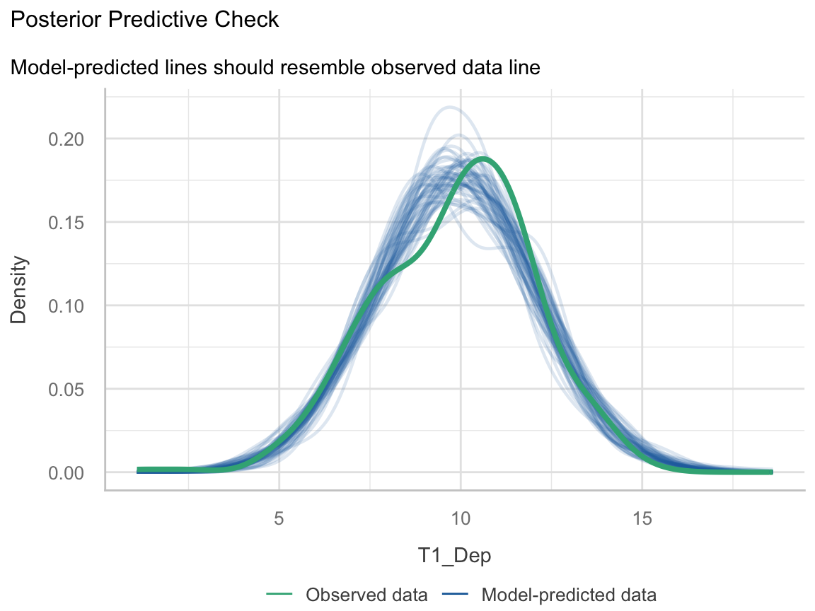
Question: If the model were true, would it produce data that look like ours?
Here: close. Depression scores are a little more peaked than the model expects, but nothing alarming.
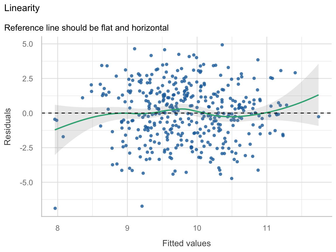
Question: Is the straight line the right shape?
Here: flat. ✅
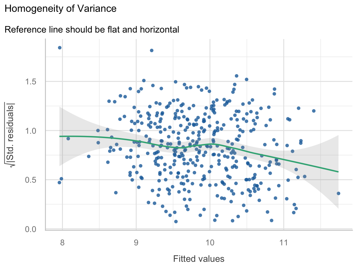
Question: Is the model equally wrong for everyone?
Here: a gentle downward drift. The model misses a little less for kids with high predicted depression. Hold that thought.
Warning: Heteroscedasticity (non-constant error variance) detected (p = 0.016).
The plot says “slight.” The test says “significant.” With 400 people, the test can detect a slight tilt. Whether that tilt matters is a separate question.
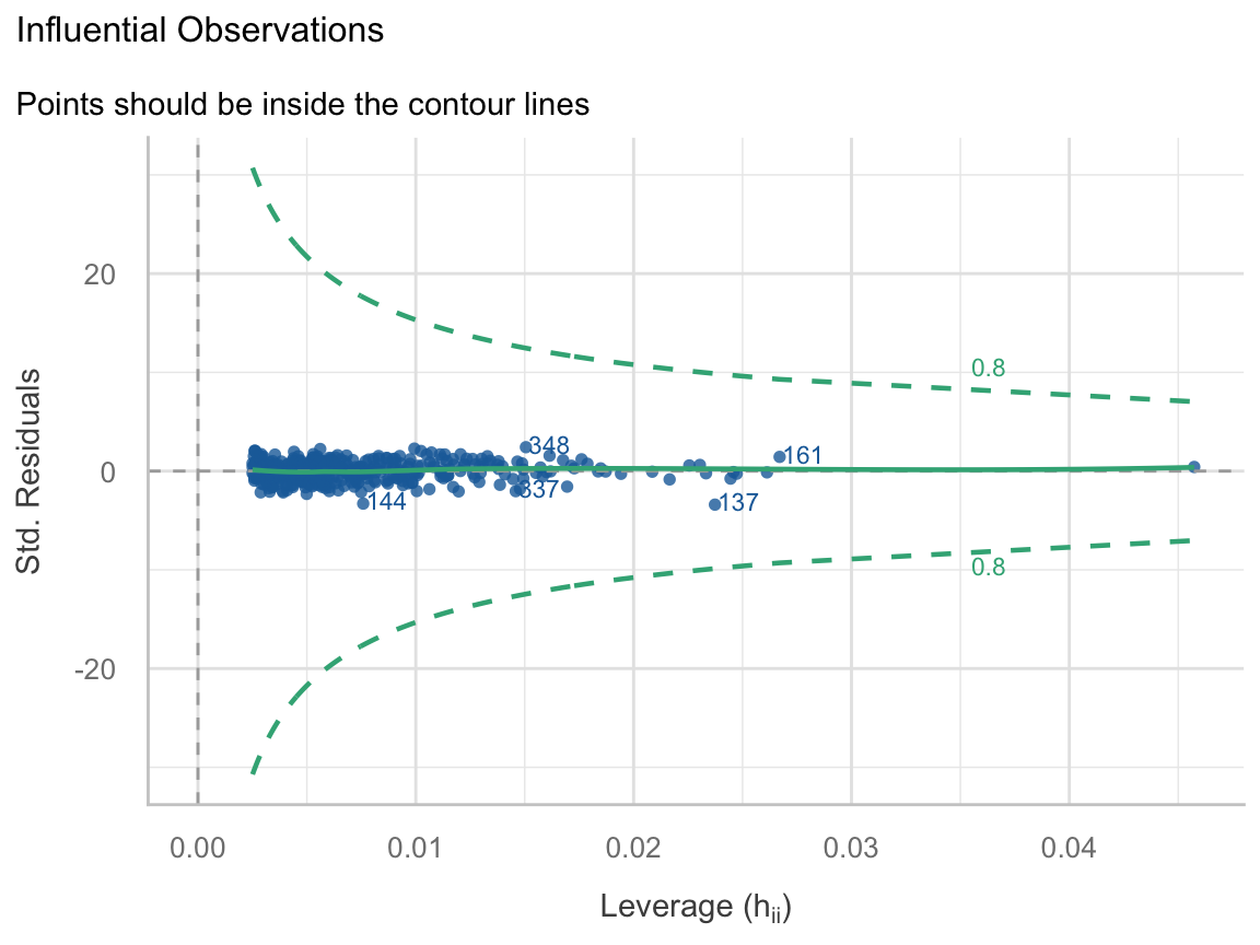
Question: Is any single person running the model?
Here: nobody close. ✅
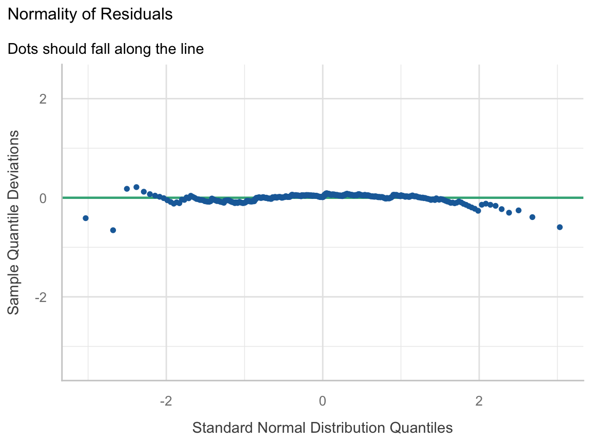
Question: Are the leftovers roughly bell-shaped?
Here: fine. ✅ And with n = 400, the Central Limit Theorem covers a lot of sins here.
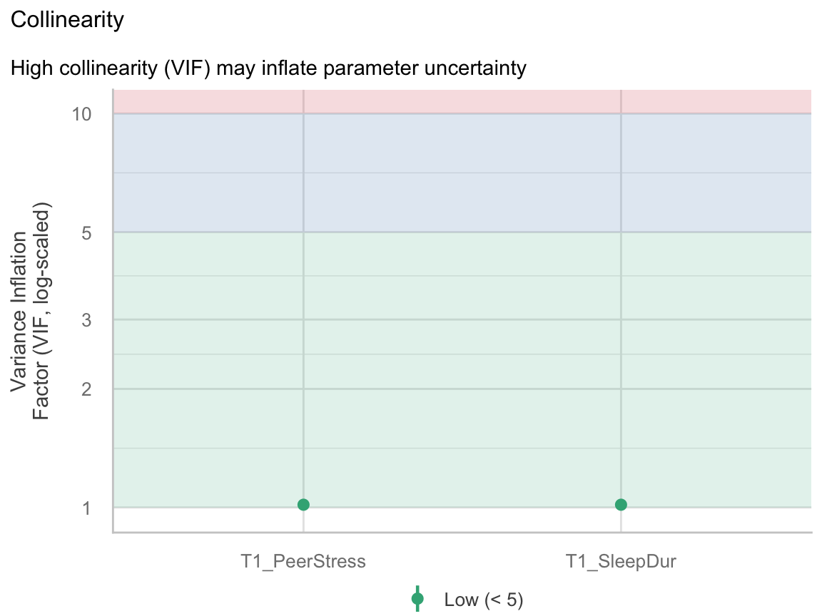
Question: Are the predictors stepping on each other? (Week 8)
Here: VIF = 1.02. Sleep and peer stress barely overlap (r = −.13). ✅
fit_two| Panel | Verdict |
|---|---|
| PP check | ✅ Close enough |
| Linearity | ✅ Flat |
| Equal variance | ⚠️ Slight drift; robust SEs barely differ |
| Influence | ✅ Nobody outside the contours |
| Normality | ✅ Fine |
| Collinearity | ✅ VIF ≈ 1 |
Week 7’s interpretation stands. Most of the time, this is what diagnostics look like. You check, the model is fine, you write one sentence saying so, and you move on.
Tip
Week 10 Exercises · ~25 min · Pairs
Last week’s Part C, finished properly. Pick a seed, write it on the board, render. Then run check_model() on your interaction model and go panel by panel.
Bring last week’s week9_reproducibility.qmd. If you don’t have it, the activity has a catch-up chunk.
Week 7 activity: 952 popular Spotify songs. Four audio features explained about 1% of streams. Playlists explained 62%.
spotify <- import(here("files", "data", "popular_spotify.csv")) %>%
janitor::clean_names() %>%
mutate(streams = as.numeric(streams),
streams_m = streams / 1e6, # millions of streams
playlists_k = in_spotify_playlists / 1000) # thousands of playlists
fit_raw <- lm(streams_m ~ playlists_k, data = spotify)
glance(fit_raw) %>% select(r.squared, sigma, nobs)# A tibble: 1 × 3
r.squared sigma nobs
<dbl> <dbl> <int>
1 0.624 348. 952
A great model by psychology standards. Let’s look at it.
An R² of .62 told us none of this.
p1 <- spotify %>%
ggplot(aes(x = streams_m)) +
geom_histogram(bins = 40, fill = "grey60", color = "white") +
labs(x = "Streams (millions)", y = "Songs", title = "Raw") +
theme_bw(base_size = 15)
p2 <- spotify %>%
ggplot(aes(x = log10(streams))) +
geom_histogram(bins = 40, fill = "grey60", color = "white") +
labs(x = "log10(streams)", y = "Songs", title = "Logged") +
theme_bw(base_size = 15)
p1 + p2
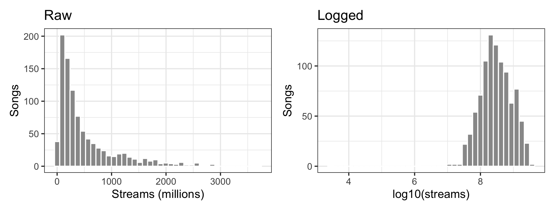
A song going from 1M to 2M streams is the same kind of change as 500M to 1,000M: it doubled. Counts like this (streams, income, reaction times, followers, reported drinks) usually behave better on a log scale.
Both streams and playlists are skewed counts, so log both.
# A tibble: 2 × 5
term estimate std.error statistic p.value
<chr> <dbl> <dbl> <dbl> <dbl>
1 (Intercept) 6.20 0.0586 106. 0
2 log_playlists 0.678 0.0172 39.3 1.73e-201
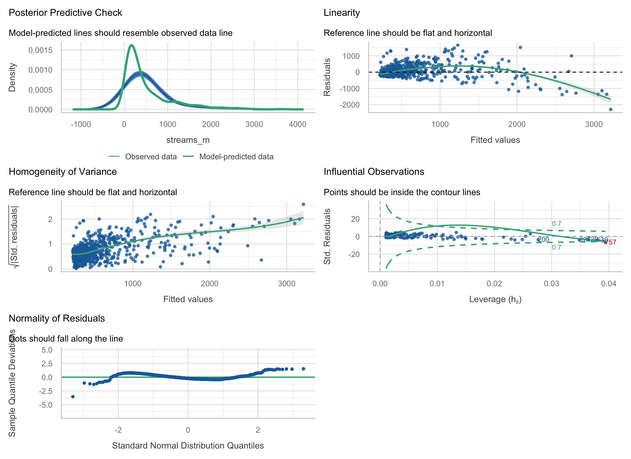
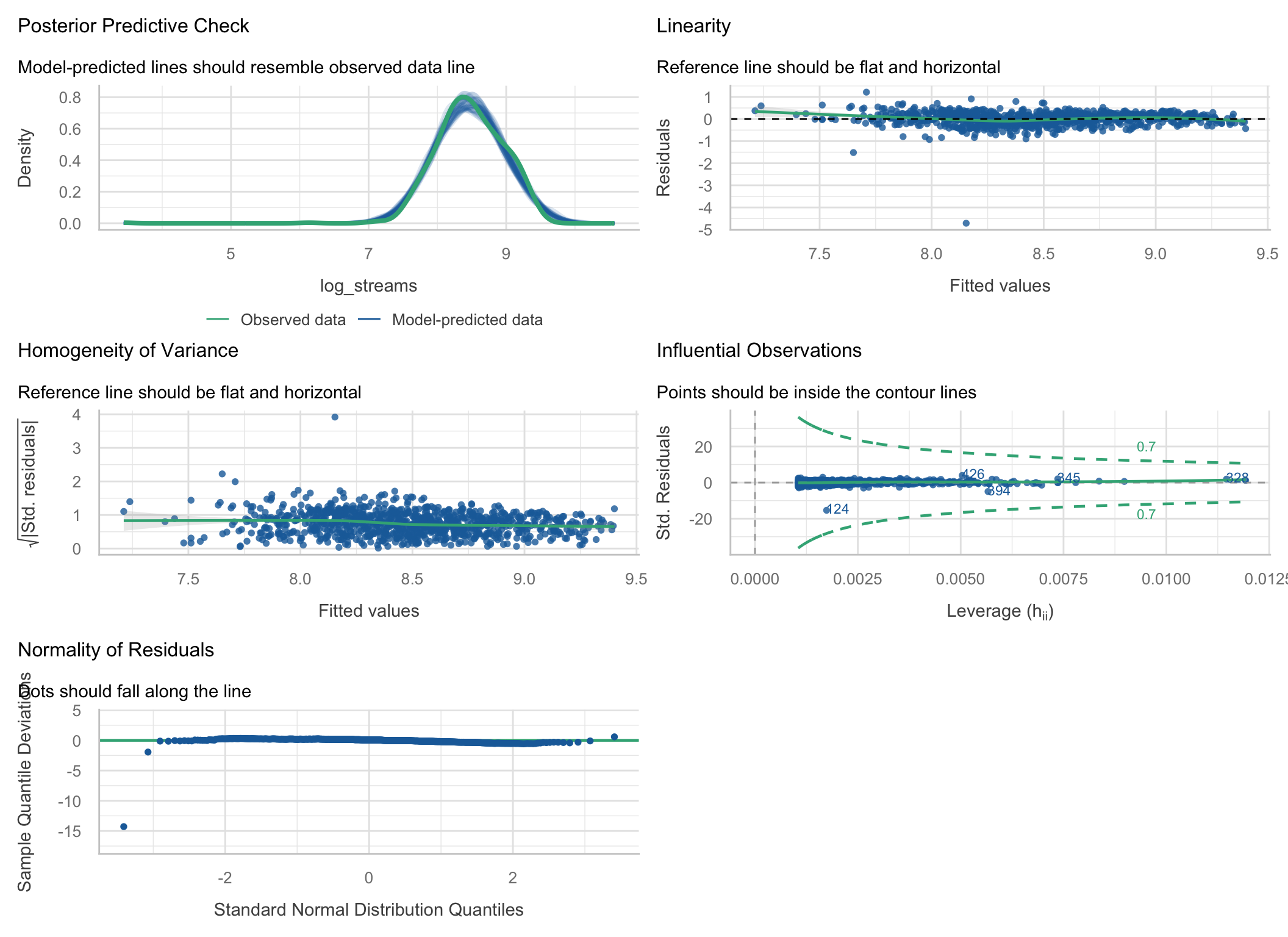
Flat lines, an even band, a bell-shaped PP check, nobody near the contours. Except one point. We’ll get to it.
# A tibble: 2 × 3
model r.squared adj.r.squared
<chr> <dbl> <dbl>
1 raw 0.624 0.623
2 logged 0.619 0.619
The fit did not improve. It went from .624 to .619.
Note
Diagnostics are not about squeezing out more R². They are about whether the coefficients, SEs, and p-values you report mean what you say they mean. The raw model was confidently wrong about the songs that matter most; the logged one is not.
log_playlists
0.6775028
log_playlists
4.758859
That sentence was impossible to say from the raw model, which claimed every 1,000 playlists added a flat 57 million streams to every song.
That lone point in the logged model:
# A tibble: 3 × 4
track_name streams in_spotify_playlists .std.resid
<chr> <dbl> <int> <dbl>
1 Que Vuelvas 2762 763 -15.4
2 Jhoome Jo Pathaan 1365184 138 -4.95
3 QUEMA 11599388 437 -3.02
2,762 streams for a song on 763 playlists. A standardized residual of −15: about 52,000 times fewer streams than the model predicts.
Drop that song and re-run the formal tests on 951 songs:
Warning: Non-normality of residuals detected (p < .001).
Warning: Heteroscedasticity (non-constant error variance) detected (p < .001).
The plots look fine. Both tests say “violated.” Who’s right?
A significance test asks “can I detect any departure at all?” That depends on n, not on whether the departure matters.
set.seed(640)
# Small sample, badly skewed errors
p_small <- replicate(1000, {
x <- rnorm(15); y <- x + (rexp(15) - 1)
shapiro.test(resid(lm(y ~ x)))$p.value
})
# Huge sample, nearly normal errors (t with 10 df)
p_big <- replicate(200, {
x <- rnorm(5000); y <- x + rt(5000, df = 10)
shapiro.test(resid(lm(y ~ x)))$p.value
})
x <- rnorm(15); y <- x + (rexp(15) - 1)
q1 <- tibble(r = resid(lm(y ~ x))) %>%
ggplot(aes(sample = r)) + stat_qq() + stat_qq_line() +
labs(title = paste0("n = 15, badly skewed\nflagged in ",
round(100 * mean(p_small < .05)), "% of samples")) +
theme_bw(base_size = 14)
x <- rnorm(5000); y <- x + rt(5000, df = 10)
q2 <- tibble(r = resid(lm(y ~ x))) %>%
ggplot(aes(sample = r)) + stat_qq(alpha = .2) + stat_qq_line() +
labs(title = paste0("n = 5,000, nearly normal\nflagged in ",
round(100 * mean(p_big < .05)), "% of samples")) +
theme_bw(base_size = 14)
q1 + q2
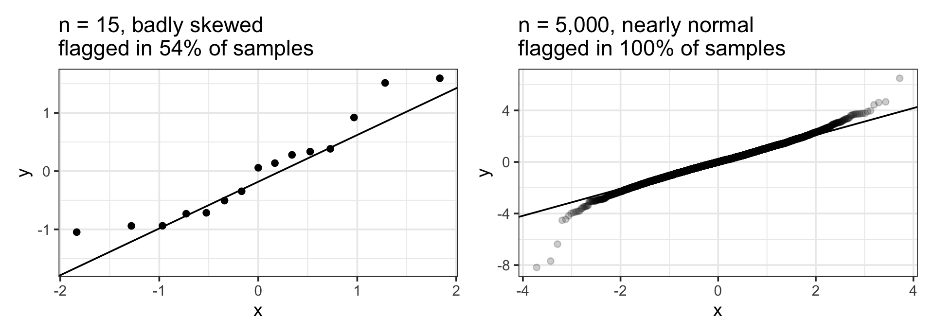
Small samples: real problems slip through. Large samples: harmless wiggles get flagged. Look at the plots. Use the tests as a second opinion, never as the verdict.
Back to the raw model. Case 757 was outside the contour:
# A tibble: 3 × 5
track_name streams_m playlists_k .hat .cooksd
<chr> <dbl> <dbl> <dbl> <dbl>
1 Get Lucky - Radio Edit 934. 52.9 0.0394 0.919
2 Mr. Brightside 1807. 52.0 0.0379 0.312
3 Smells Like Teen Spirit - Remastered 2021 1690. 50.0 0.0348 0.287
Get Lucky is on more playlists than any other song in the data (52,898), but has “only” 934M streams.
.hat): unusual on the predictors. Most playlists of anyone.cooksd): leverage × residual. How much every prediction would shift if this one case vanished# A tibble: 2 × 3
`Get Lucky` estimate std.error
<chr> <dbl> <dbl>
1 with 56.7 1.43
2 without 58.6 1.42
One song out of 952 moved the slope by about 2 million streams per thousand playlists. Not a disaster here, but in a sample of 40 one case can flip a sign.
Warning
Never delete points to get to p < .05. “Removed outliers” with no rule and no with-and-without comparison is a red flag to every reviewer.
Songs are on playlists on Spotify, Apple, and Deezer. Each one alone predicts streams.
# Correlation Matrix (pearson-method)
Parameter | deezer_playlists | in_apple_playlists | in_spotify_playlists
-----------------------------------------------------------------------------------
streams_m | 0.60*** | 0.77*** | 0.79***
in_spotify_playlists | 0.83*** | 0.71*** |
in_apple_playlists | 0.47*** | |
p-value adjustment method: Holm (1979)
# A tibble: 4 × 5
term estimate std.error statistic p.value
<chr> <dbl> <dbl> <dbl> <dbl>
1 (Intercept) 141. 12.8 11.0 1.56e-26
2 in_spotify_playlists 0.0365 0.00288 12.7 4.00e-34
3 in_apple_playlists 2.77 0.168 16.5 1.04e-53
4 deezer_playlists -0.0107 0.0161 -0.666 5.05e- 1
Deezer playlists correlate r = .60 with streams on their own. In this model, the Deezer coefficient is negative and not significant.
Deezer didn’t stop mattering. It correlates r = .83 with Spotify playlists, so once Spotify is in the model there is almost nothing left for Deezer to explain, and the model can’t tell the two apart.
# Check for Multicollinearity
Low Correlation
Term VIF adj. VIF
in_apple_playlists 2.18 1.48
deezer_playlists 3.43 1.85
Moderate Correlation
Term VIF adj. VIF
in_spotify_playlists 5.35 2.31
SE_factor column)What to do: ask whether you need all three. Pick the one your question is about, or combine them (e.g., average their z-scores into one “popularity” score). If you only care about prediction, collinearity barely matters.
Interactions create collinearity: study × tutor is built out of study and tutor.
tutor <- import(here("files", "data", "tutor.csv")) %>%
mutate(tutor_f = factor(tutor, levels = c(0, 1), labels = c("No tutor", "Tutor")),
study_c = study - mean(study))
vif_raw <- check_collinearity(lm(grade ~ study * tutor_f, data = tutor))
vif_cen <- check_collinearity(lm(grade ~ study_c * tutor_f, data = tutor))
tibble(term = c("study", "tutor", "study × tutor"),
uncentered = round(vif_raw$VIF, 2),
centered = round(vif_cen$VIF, 2))# A tibble: 3 × 3
term uncentered centered
<chr> <dbl> <dbl>
1 study 2.7 2.7
2 tutor 7.52 1.36
3 study × tutor 11.4 2.34
Same model, same interaction test. Centering took the interaction’s VIF from about 11 down to about 2. A high VIF on an uncentered interaction is not a reason to panic. Center, then check.
ASAP measured each adolescent three times. Stack the three waves and fit one regression:
[1] 1076
[1] 400
The model thinks it has 1076 independent observations. It has 400 kids.
# Correlation Matrix (pearson-method)
Parameter | T3 | T2
-----------------------------
T1 | 0.18** | 0.35***
T2 | 0.47*** |
p-value adjustment method: Holm (1979)
If the model underpredicts a kid at T2, it probably underpredicts them at T3 too. The errors are not independent, so the SEs are too small and the p-values too optimistic.
Note
check_model() cannot catch this. Independence is a design question: repeated measures, siblings, students in classrooms, therapy clients with the same therapist. The fix is a multilevel model.
Tip
~10 min · Same pairs, same seed
Does your conclusion hold up? Refit your interaction three ways: robust SEs, dropping cases with Cook’s distance > 4/n, and one version with last week’s TIPI-zeros mistake left in.
| Problem | How you see it | What to do |
|---|---|---|
| Nonlinearity | Curved line in Linearity panel | Log or other transform; add a squared term; rethink the model |
| Unequal variance | Rising line / funnel | Log the outcome if it’s a skewed count; robust SEs (vcov = "HC3") |
| Non-normal residuals | S-curve or peeled tails in Q-Q | Large n: usually ignore. Small n: transform, or bootstrap CIs |
| Influential case | Point outside the Cook’s contours | Check for errors; fit with and without; report both |
| Collinearity | VIF > 5–10 | Center interactions; drop or combine overlapping predictors |
| Non-independence | Your design, not a plot | Multilevel model (Week 13) |
That last one is the analysis-plan habit. You will need it for the final project.
Model assumptions were evaluated with residual diagnostics (
performance::check_model()). In the untransformed model, residuals showed marked curvature, increasing variance with fitted values, and right skew, so both streams and playlist counts were log10-transformed. The transformed model showed no evidence of nonlinearity, heteroscedasticity, or influential observations, with one exception: a single song (2,762 streams) had a standardized residual of −15.4, was judged a data-entry error, and was excluded (N = 951). Each tenfold increase in playlist count was associated with a 4.7-fold increase in streams, b = 0.67, 95% CI [0.64, 0.70], R² = .68.
Tip
Say what you checked, what you found, what you did, and why. If everything looked fine, one sentence is enough: “Residual diagnostics showed no evidence of nonlinearity, heteroscedasticity, non-normality, or influential observations.”
Tip
~15 min · Write, render, tally
The same analysis on 1,000 different seeds, instead of the 15 on the board:
| Version | Seeds with p < .05 |
|---|---|
| Original | 21.6% |
| Robust SEs | 26.7% |
| Drop Cook’s > 4/n | 19.7% |
| TIPI zeros left in (the mistake) | 23.1% |
All 33,982 usable responses:
The interaction is real and tiny. With n ≈ 340, about one sample in five can see it, and which version of the analysis you run decides a fifth of the verdicts.
Reproducible (it renders) is not robust (it survives other defensible choices), and neither is replicable (a new sample agrees). Diagnostics tell you which choices to check. Reporting them lets the next person check you.
Tip
~10 min · Pairs
Each panel comes from a different model. For each one: which assumption, what’s wrong, what would you do?
set.seed(1029)
n <- 250
x <- runif(n, 1, 10)
mA <- lm(y ~ x, data = tibble(x, y = 2 + 3 * x - 0.3 * x^2 + rnorm(n, 0, 1.5)))
mB <- lm(y ~ x, data = tibble(x, y = exp(0.3 * x + rnorm(n, 0, 0.45))))
dC <- tibble(x = c(x[1:39], 25), y = c(2 + 0.5 * x[1:39] + rnorm(39, 0, 1.5), -4))
mC <- lm(y ~ x, data = dC)
x1 <- rnorm(n); x2 <- x1 + rnorm(n, 0, 0.2); x3 <- rnorm(n)
mD <- lm(y ~ x1 + x2 + x3, data = tibble(x1, x2, x3, y = x1 + x3 + rnorm(n)))
pA <- plot(check_model(mA, check = "linearity", panel = FALSE))[[1]] + labs(title = "A")
pB <- plot(check_model(mB, check = "qq", panel = FALSE))[[1]] + labs(title = "B")
pC <- plot(check_model(mC, check = "outliers", panel = FALSE))[[1]] + labs(title = "C")
pD <- plot(check_model(mD, check = "vif", panel = FALSE))[[1]] + labs(title = "D")
(pA + pB) / (pC + pD)
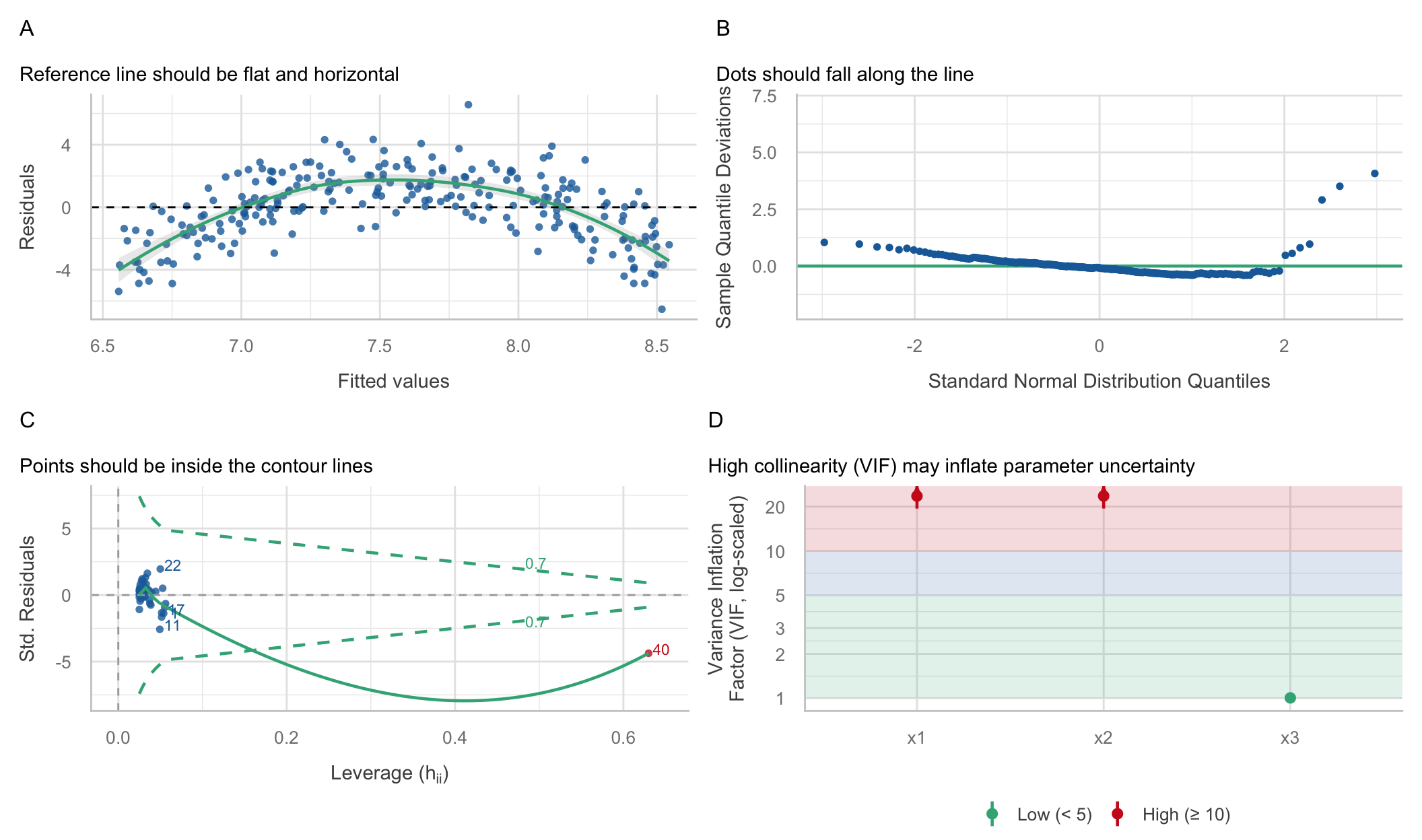

x, then re-check.x and a big miss, outside the Cook’s contour, in a sample of only 40. Check it, then fit with and without.x1 and x2 are near copies (VIF way above 10). Keep the one your question is about, or combine them.Notice what’s not on this slide: independence. No panel would have shown it.
Finish these in your notes:
📋 Lab 9 — Groups, Slopes & Interactions, due Tuesday 11/3 at 11:59pm
📖 Readings for Missing Data + Model Building/Comparison:
💾 Class Check next week
📂 Final Project — posted Friday
The final project will be up on the website Friday. It uses everything from today: you’ll write an assumption-check plan before you run your confirmatory model. Read it over the weekend.