Week 12: Categorical & Logistic Regression
Date: November 10, 2025
Today…
Final Project Prep
Some helpful tools (autosave & new library)
Regression Review
Categorical Predictors Review
Logistic Regression
Model Diagnostics 🤷
Autosave
Tools >> Global Options >> Code >> Saving

New Library: genzplyr

dplyr but make it bussin fr fr no cap
Regression does a vibe check on the data. lowkey draw a line through the points.
Regression
What is the equation for a regression??
Regression
\[ Y_i = b_0 + b_1X_{1i} + b_2X_{2i} + ... + b_nX_{ni}+ e_i \]
Regression
How do we interpret the regression coefficients (Intercepts & slopes)?
Regression
INTERCEPT: When all predictor variables are set to 0, our expected value (predicted \(\hat{Y}\)) will be this value.
SLOPES: For every 1 unit change in our \(X_n\) variable, there will be beta (b or \(\beta\)) units increase in our Y (outcome) variable, holding all other variables constant.
Explaining Variance
Explaining Variance
What do we do with categorical variables as predictors?

Categorical Predictors = factors
Typically identified by a grouping variable that may be a character
chr [1:1000] "Democrat" "Democrat" "Independent" "Republican" "Democrat" ...Need to change the variable from character to factor which will assign a number to each group
Dummy Coding (replacing factors)
Numerical placeholders used to represent categorical variables
Taking a categorical variable with \(k\) levels (e.g., Democratic, Independent, Republican) into \(k-1\) binary variables.
| political_affiliation | becomes | Ind (binary1) | Rep (binary2) |
|---|---|---|---|
| Democrat | –> | 0 | 0 |
| Independent | –> | 1 | 0 |
| Republican | –> | 0 | 1 |
| … | … | … |
Dummy Coding
For the variable with \(k\) levels, we use \(k-1\) binary variables…why not use all of them?
Including all three variables would result in perfect multicollinearity. All Democrats would be related to other Democrats and unrelated to everything else
By including 2 binary variables, we are able to obtain all information about group membership
Dummy Coding
The group that has 0’s for all the binary variables is the reference group
For interpretation, we will make our statements in reference to this group
| political_affiliation | becomes | Ind (binary1) | Rep (binary2) |
|---|---|---|---|
| Democrat | –> | 0 | 0 |
| Independent | –> | 1 | 0 |
| Republican | –> | 0 | 1 |
| … | … | … |
Categorical Regression
Going back to our Transformers dataset, let’s see how our political affiliation variable can predict # of transformers movies
Usually you have to create the separate dummy variables, but not in R. As long as your predictor is set as a factor, R will automatically dummy code the variable.
You can also double check the dummy/contrast coding
Interpretation
We are shown the different levels of our predictor variable, but you will not see a predictor for the reference group…this is the intercept!
Every interpretation is ALWAYS in reference to the reference group
Go to next slide for a pretty table
Call:
lm(formula = transformers ~ pol, data = cah_data)

Residuals:
    Min      1Q  Median      3Q     Max
-1.3447 -1.1804 -0.3447  0.8196  3.8367

Coefficients:
               Estimate Std. Error t value            Pr(>|t|)
(Intercept)     1.18039    0.09399  12.559 <0.0000000000000002 ***
polIndependent  0.16434    0.12349   1.331               0.184
polRepublican  -0.01713    0.14257  -0.120               0.904
---
Signif. codes:  0 '***' 0.001 '**' 0.01 '*' 0.05 '.' 0.1 ' ' 1

Residual standard error: 1.501 on 799 degrees of freedom
  (198 observations deleted due to missingness)
Multiple R-squared:  0.003244,  Adjusted R-squared:  0.0007487
F-statistic:   1.3 on 2 and 799 DF,  p-value: 0.2731
Interpretation
Interpretation (text)
A linear regression investigated the relationship between political affiliation and number of transformers movies watched. Democrats showed a significant difference from 0 (b = 1.18, p < .001), but there was not a significant difference between Democrats and Independents (p = .18) or Democrats and Republicans (p = .90). The findings suggest that there are no significant differences between groups.
Note
How does this sound?
Changing the Reference Group
Maybe we want to compare to a specific group
We need to then update the reference group
Call:
lm(formula = transformers ~ pol2, data = cah_data)

Residuals:
    Min      1Q  Median      3Q     Max
-1.3447 -1.1804 -0.3447  0.8196  3.8367

Coefficients:
               Estimate Std. Error t value            Pr(>|t|)
(Intercept)     1.34473    0.08011  16.786 <0.0000000000000002 ***
pol2Democrat   -0.16434    0.12349  -1.331               0.184
pol2Republican -0.18146    0.13383  -1.356               0.175
---
Signif. codes:  0 '***' 0.001 '**' 0.01 '*' 0.05 '.' 0.1 ' ' 1

Residual standard error: 1.501 on 799 degrees of freedom
  (198 observations deleted due to missingness)
Multiple R-squared:  0.003244,  Adjusted R-squared:  0.0007487
F-statistic:   1.3 on 2 and 799 DF,  p-value: 0.2731
lm() or aov() ?
We have the same setup between a linear model and a one-way ANOVA.
\[ Outcome_{continuous} = Predictor_{categorical} + error \]
Why would we pick one over another?
If we have a reason to have a reference group –> Regression
- Maybe we have a control group
If we just expect a difference somewhere –> ANOVA
- When you are predicting # movies from political affiliation
Everything is a linear model

Break ☕🍵🥐
Categories in Action (last time)
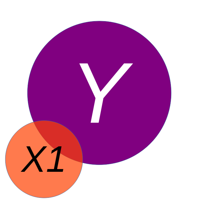
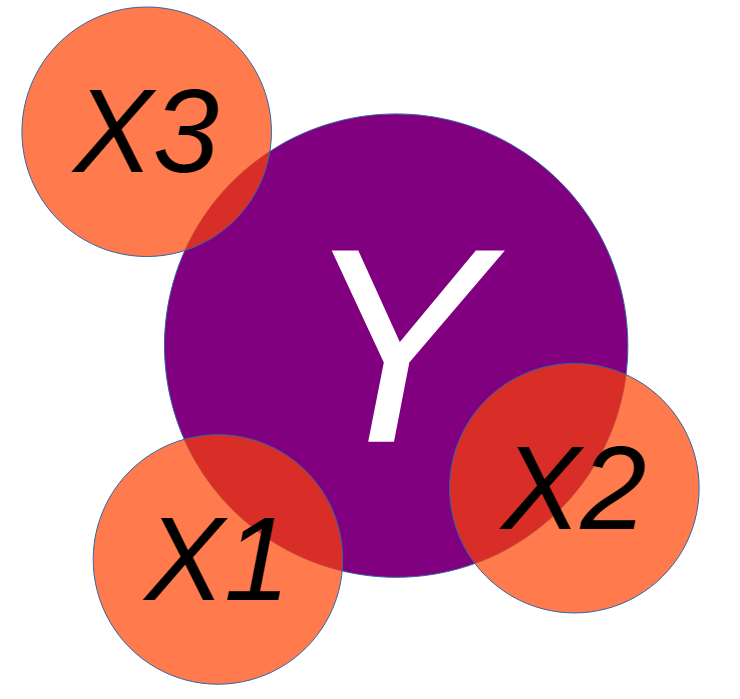
Goal: Gain greater familiarity with dummy coding and categorical predictors
Scenario: We are researchers examining the impact of a new intervention on reducing the vocalization “6️⃣7️⃣” in the youths. We have done classroom observations to collect data on how many times students say “6️⃣7️⃣” after receiving the intervention. Youths have been randomly assigned to one of 3 groups, and we need to determine which had the biggest impact.
Run the Regression with complete data
Note
Dr. Haraden needs to write the equation on the board 🧑🏫 Calculate the expected value for each group
Call:
lm(formula = post_score ~ group, data = six_seven)

Residuals:
   Min     1Q Median     3Q    Max
-5.000 -2.375  0.000  1.500  7.000

Coefficients:
            Estimate Std. Error t value         Pr(>|t|)
(Intercept)  11.5000     0.9487  12.122 0.00000000000197 ***
groupOrange   1.5000     1.3416   1.118           0.2734
groupYellow   3.0000     1.3416   2.236           0.0338 *
---
Signif. codes:  0 '***' 0.001 '**' 0.01 '*' 0.05 '.' 0.1 ' ' 1

Residual standard error: 3 on 27 degrees of freedom
Multiple R-squared:  0.1562,    Adjusted R-squared:  0.09375
F-statistic:   2.5 on 2 and 27 DF,  p-value: 0.1009
Now what are the means for each group?
Now what are the means for each group?
Using R
Import dataset, include age and pre-scores to see how that changes interpretation
Warning
Dr. Haraden is going to start opening up R and doing a follow-along thing. You have been warned
Everything is a linear model

Introducing Generalized Linear Model
6️⃣7️⃣ Status
In our last example, we were able to see how these categorical variables could predict a continuous variable. This is perfect for linear regression.
What if we want to see if students have “recovered” from 6️⃣7️⃣?
We would then ask: “Which participants dropped below the clinical threshold for 6️⃣7️⃣ at follow-up? Now, our outcome is either recovered or not recovered.”
Recovery Status
Now we have a binary outcome; Yes/No recovery
What happens when we fit a linear regression? What are the chances of someone with a pre-score of 12 recovering by the follow-up?
Recovery Status
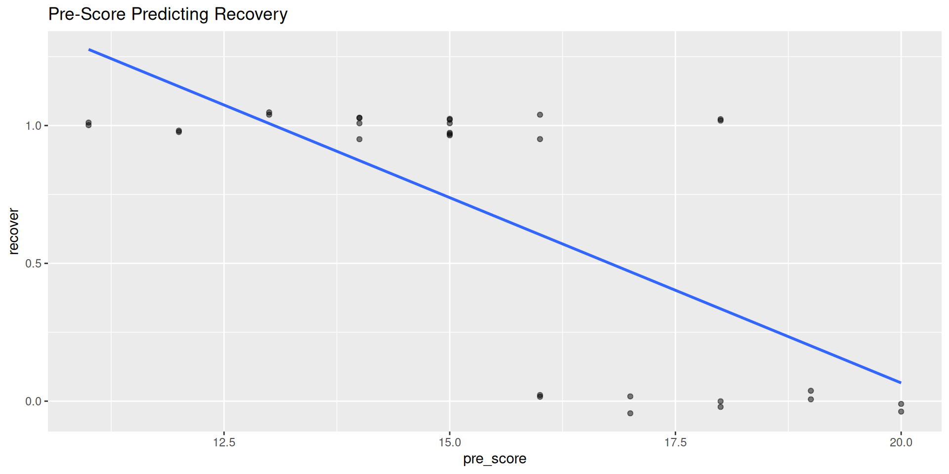
Binary Outcomes in Regression
A simple line is not going to appropriately capture the data
- Plus, it definitely doesn’t make it a normal distribution! We only have 2 scores in our predictor variable…
Introducing Logistic Regression 🌟
- Using a logistic function we are able to better capture the data and get a “likelihood” or “probability” of an outcome
Probability to Odds to Log-Odds
Probability (p): The chance of an event happening. Ranges from 0 to 1
Odds: The ratio of the probability of an event happening to it not happening.
\(Odds = \frac{p}{1-p}\)
Ranges from 0 to ∞. An odds of 4 means the event is 4 times more likely to happen than not.
Log-Odds (logit): The natural log of the odds
\(Logit(p) = ln(\frac{p}{1-p})\)
Ranges from -∞ to +∞
Important
This step transforms our bounded outcome variable (0/1) to an unbound one!
Generalized Linear Model (GLM)
A generalization of a linear model (duh) that is used when the response variable has a non-normal error distribution
Most commonly used when there is a binary (0-1) or count variable as the outcome (we will focus on the binary)
Ultimately, we are trying to identify the probability of the outcome taking the value 1 (“success”) that is being modeled in relation to the predictor variables
GLM: Logistic Regression
\[ transformation(p_i)=\beta_0+\beta_1x_{1,i} + \beta_2x_{2,i} + \cdots+\beta_lx_{k,i} \]
We have to apply a transformation to the left side so that it can take variables beyond just 0 & 1
A common transformation is the \(logit\ transformation\)
\[ \log_{e}\left( \frac{p_i}{1-p_i} \right) = \beta_0 + \beta_1 x_{1,i} + \beta_2 x_{2,i} + \cdots + \beta_k x_{k,i} \]
Recovering from 6️⃣7️⃣
Now we have a tool to figure this out, let’s see if the pre-score can predict recovery!
GLM - 6️⃣7️⃣ Data Interpretation
Note
Interpretation is still the same as linear regression, except we are dealing with log-odds of the outcome. What does that mean??
Call:
glm(formula = recover ~ pre_score, family = "binomial", data = six_seven)

Coefficients:
            Estimate Std. Error z value Pr(>|z|)
(Intercept)  20.1873     7.0700   2.855  0.00430 **
pre_score    -1.2002     0.4268  -2.812  0.00492 **
---
Signif. codes:  0 '***' 0.001 '**' 0.01 '*' 0.05 '.' 0.1 ' ' 1

(Dispersion parameter for binomial family taken to be 1)

    Null deviance: 38.191  on 29  degrees of freedom
Residual deviance: 18.216  on 28  degrees of freedom
AIC: 22.216

Number of Fisher Scoring iterations: 6
GLM - 6️⃣7️⃣ Data Interpretation (tables)
We want to be able to interpret these coefficients more easily so we put them into Odds Ratios
sjPlot is always coming in with the good tables
Odds Ratios (OR)
OR > 1: The predictor increases the odds of the outcome. (e.g., OR of 2.5 means the odds of believing in ghosts are 2.5 times higher).
OR < 1: The predictor decreases the odds of the outcome. (e.g., OR of 0.4 means the odds of believing in ghosts are 60% lower).
OR = 1: The predictor has no effect on the odds of the outcome.
Visualization
Extract the model implied probabilities for each individual
Plotting the predicted probabilities
probs %>%
ggplot(aes(pre_score, .fitted)) +
  geom_line(color = "blue", linewidth = 0.5) +
  geom_jitter(width = 0.2, alpha = 0.5) +
  labs(
    title = "Predicted Probability of Recovery from 6-7 by Pre-Score",
    x = "Pre-Score",
    y = "Predicted Probability of Recovery"
  ) +
  ylim(0, 1) + # Keep the y-axis bounded at 0 and 1
  theme_minimal()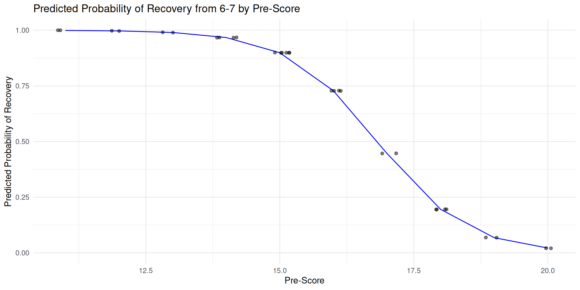
Logistic Regression: Summary
| Feature | Linear Regression | Logistic Regression |
|---|---|---|
| Outcome Variable | Continuous | Categorical (Binary) |
| Equation | \(Y=β_0+β_1X\) | \(ln(\frac{p}{1-p})=β_0+β_1X\) |
| Key Interpretation | \(\beta_1\) is the change in the mean of Y | \(\exp(\beta_1)\) is the odds ratio |
| R Function | lm() |
glm(..., family="binomial") |
Break ☕🍵🥐
Next Up…
Follow along to apply these methods to a new dataset!
Predicting the probability of believing in ghosts. Hopefully we have time to go through this example 👻