#Don't know if I'm using all of these, but including theme here anywayslibrary(tidyverse)library(rio)library(broom)library(psych)library(gapminder)library(psychTools)#Remove Scientific Notation options(scipen=999)
Overview of Regression
Regression is a general data analytic system
Lots of things fall under the umbrella of regression
This system can handle a variety of forms of relations and types of variables
The output of regression includes both effect sizes and statistical significance
We can also incorporate multiple influences (IVs) and account for their intercorrelations
Uses for regression
Adjustment: Take into account (control) known effects in a relationship
Prediction: Develop a model based on what has happened previously to predict what will happen in the future
Explanation: examining the influence of one or more variable on some outcome
Study Design & Collection
Design - When data are collected
Retrospective/Prospective
Longitudinal
Cross-Sectional
Collection - How data are collected
Experimental
Field
Observational
Meta-analysis
Neuroimaging/Psychophysiology
Survey
Quasi-Experimental
Regression Equation
With regression, we are building a model that we think best represents the data, and the broader world
\[
Data = Model + error
\]
At the most simple form we are drawing a line to characterize the linear relationship between the variables so that for any value of x we can have an estimate of y
\[
Y = mX + b
\]
Y = Outcome Variable (DV)
m = Slope Term
X = Predictor (IV)
b = Intercept
Regression Equation
Overall, we are providing a model to give us a “best guess” on predicting
Let’s “science up” the equation a little bit:
\[
Y_i = b_0 + b_1X_i + e_i
\]
This equation is capturing how we are able to calculate each observation ( \(Y_i\) )
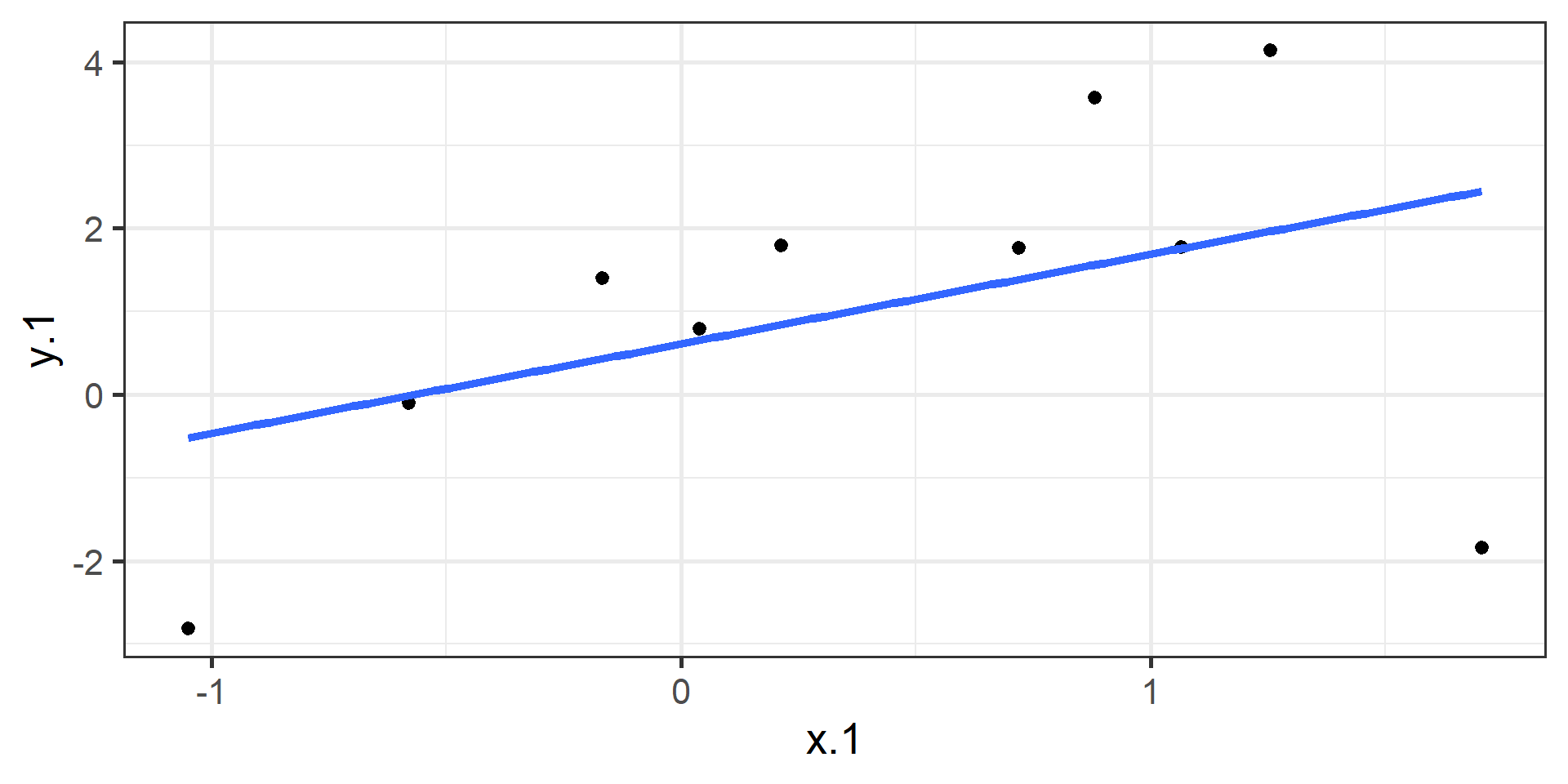
\[
\hat{Y_i} = b_0 + b_1X_i
\]
This one will give us the “best guess” or expected value of \(Y\) given \(X\)
Regression Equation
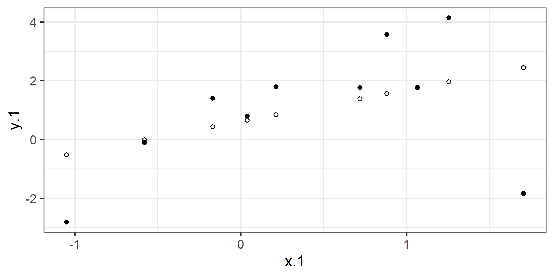
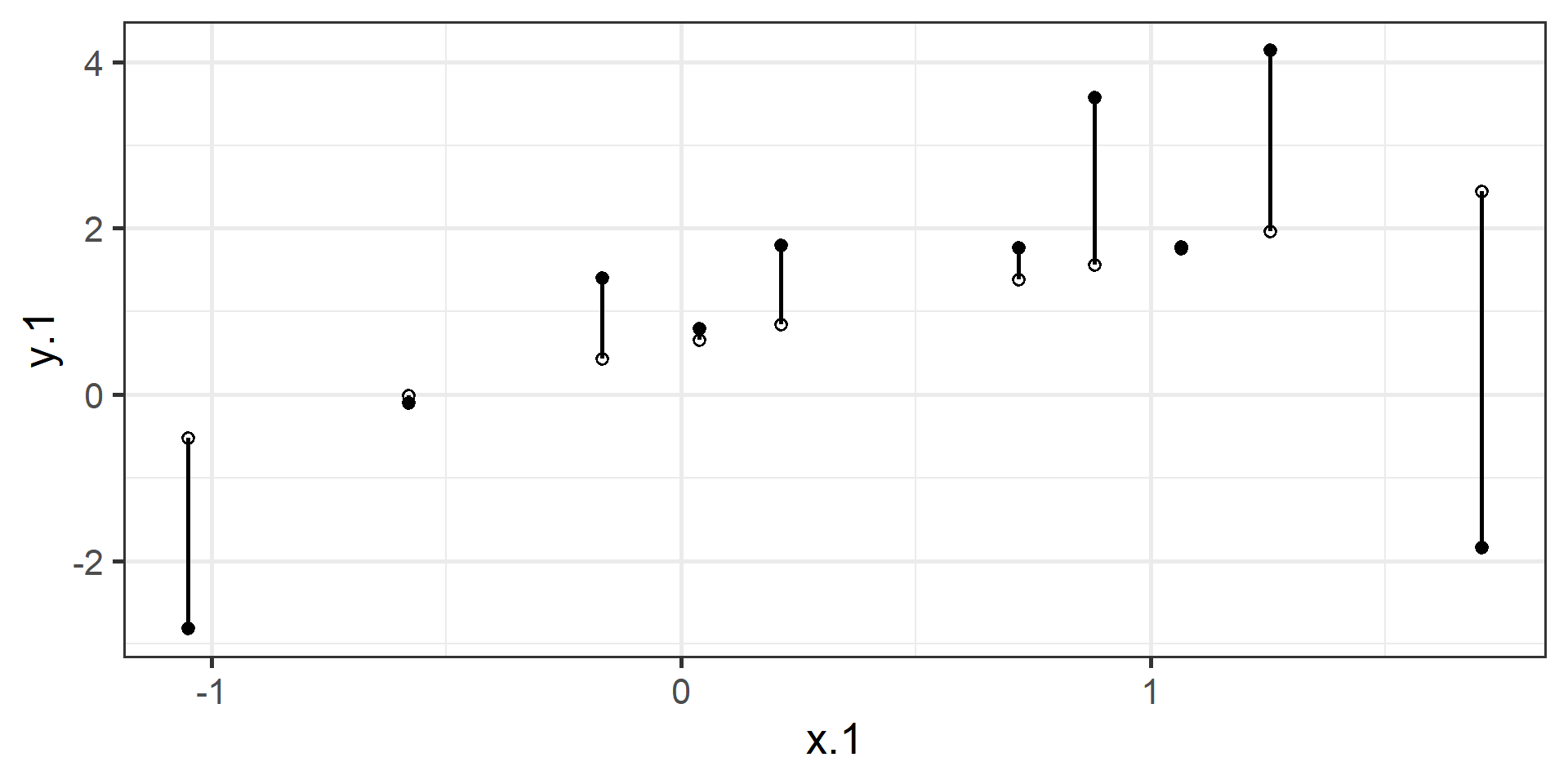
There are two ways to think about our regression equation. They’re similar to each other, but they produce different outputs. \[Y_i = b_{0} + b_{1}X_i +e_i\] \[\hat{Y_i} = b_{0} + b_{1}X_i\]
The model we are building by including new variables is to explain variance in our outcome
Note
\(\hat{Y}\) signifies the fitted score – no errorThe difference between the fitted and observed score is the residual (\(e_i\))There is a different e value for each observation in the dataset
Expected vs. Actual
\[Y_i = b_{0} + b_{1}X_i + e_i\]
\[\hat{Y_i} = b_{0} + b_{1}X_i\]
\(\hat{Y}\) signifies that there is no error. Our line is predicting that exact value. We interpret it as being “on average”
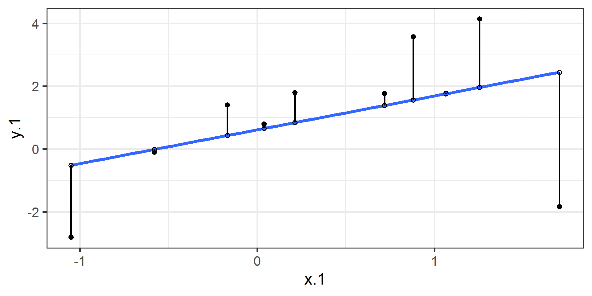
Important to identify that that \(Y_i - \hat{Y_i} = e_i\).
OLS
How do we find the regression estimates?
Ordinary Least Squares (OLS) estimation
Minimizes deviations
\[ min\sum(Y_{i} - \hat{Y} ) ^{2} \]
Other estimation procedures possible (and necessary in some cases)
In order to find the OLS solution, you could try many different coefficients \((b_0 \text{ and } b_{1})\) until you find the one with the smallest sum squared deviation. Luckily, there are simple calculations that will yield the OLS solution every time.
According to this regression equation, when \(X = 0, Y = 0\). Our interpretation of the coefficient is that a one-standard deviation increase in X is associated with a \(b_{yx}^*\) standard deviation increase in Y. Our regression coefficient is equivalent to the correlation coefficient when we have only one predictor in our model.
Estimating the intercept, \(b_0\)
intercept serves to adjust for differences in means between X and Y
otherwise, intercept is where regression line crosses the y-axis at X = 0
The intercept adjusts the location of the regression line to ensure that it runs through the point \(\large (\bar{X}, \bar{Y}).\) We can calculate this value using the equation:
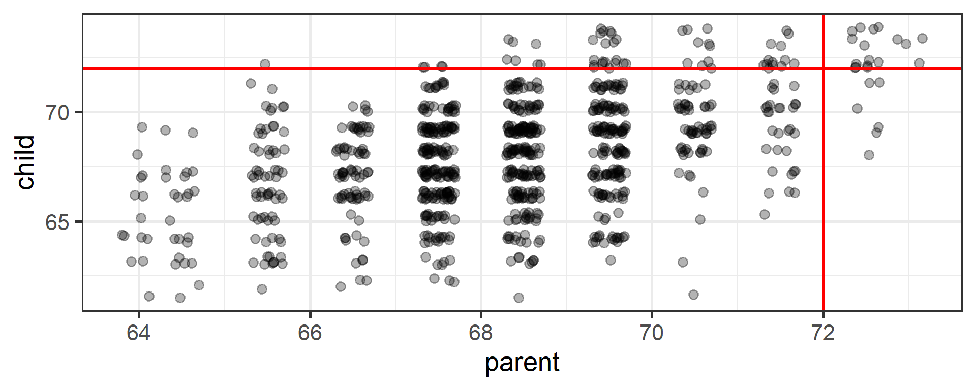
An observation about heights was part of the motivation to develop the regression equation: If you selected a parent who was exceptionally tall (or short), their child was almost always not as tall (or as short).
Code
library(psychTools)library(tidyverse)heights = psychTools::galtonmod =lm(child~parent, data = heights)point =902heights = broom::augment(mod)heights %>%ggplot(aes(x = parent, y = child)) +geom_jitter(alpha = .3) +geom_hline(aes(yintercept =72), color ="red") +geom_vline(aes(xintercept =72), color ="red") +theme_bw(base_size =20)
Regression to the mean
This phenomenon is known as regression to the mean. This describes the phenomenon in which an random variable produces an extreme score on a first measurement, but a lower score on a second measurement.
Regression to the mean
This can be a threat to internal validity if interventions are applied based on first measurement scores.
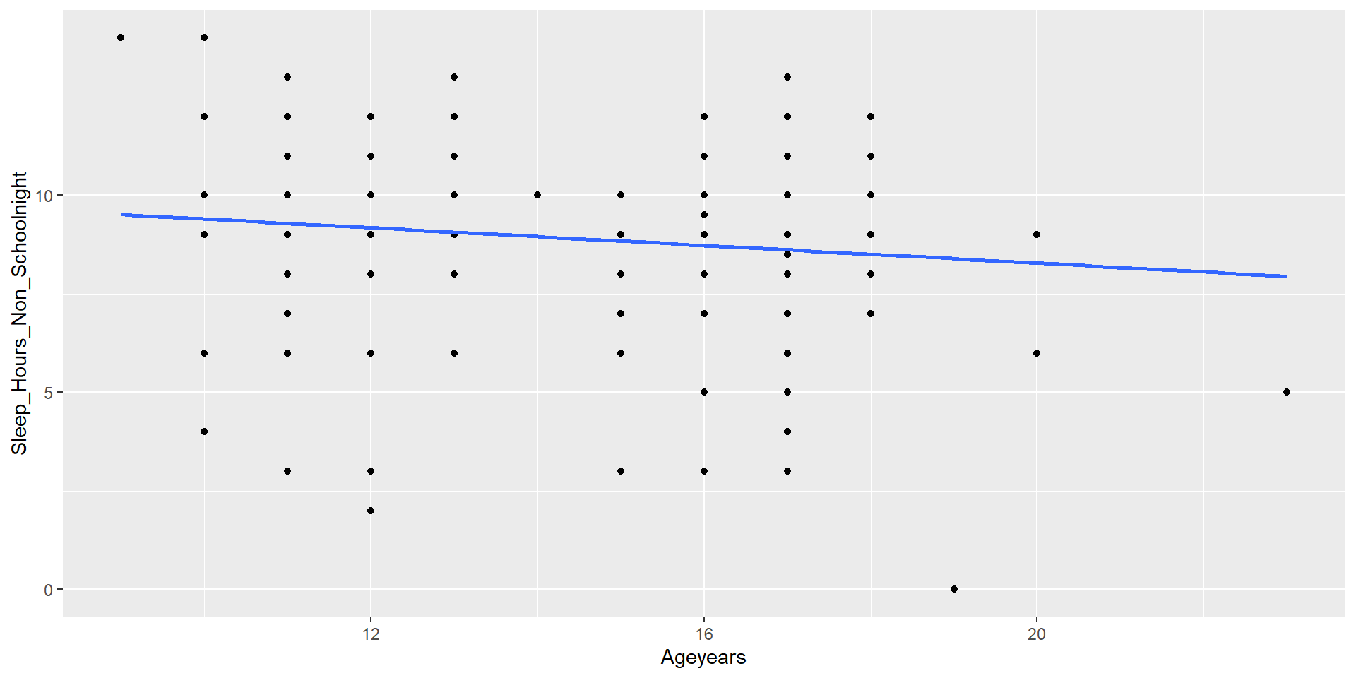
Another Dataset
school <-read_csv("https://raw.githubusercontent.com/dharaden/dharaden.github.io/main/data/example2-chisq.csv") %>%mutate(Sleep_Hours_Non_Schoolnight =as.numeric(Sleep_Hours_Non_Schoolnight)) %>%filter(Sleep_Hours_Non_Schoolnight <24) #removing impossible values
Statistical Inference
The way the world is = our model + error
How good is our model? Does it “fit” the data well?
To assess how well our model fits the data, we will examine the proportion of variance in our outcome variable that can be “explained” by our model.
To do so, we need to partition the variance into different categories. For now, we will partition it into two categories: the variability that is captured by (explained by) our model, and variability that is not.
Partitioning variation
Let’s start with the formula defining the relationship between observed \(Y\) and fitted \(\hat{Y}\):
\[Y_i = \hat{Y}_i + e_i\]
One of the properties that we love about variance is that variances are additive when two variables are independent. In other words, if we create some variable, C, by adding together two other variables, A and B, then the variance of C is equal to the sum of the variances of A and B.
Why can we use that rule in this case?
Partitioning variation
\(\hat{Y}_i\) and \(e_i\) must be independent from each other. Thus, the variance of \(Y\) is equal to the sum of the variance of \(\hat{Y}\) and \(e\).
\[\large s^2_Y = s^2_{\hat{Y}} + s^2_{e}\]
Recall that variances are sums of squares divided by N-1. Thus, all variances have the same sample size, so we can also note the following:
\[\large SS_Y = SS_{\hat{Y}} + SS_{\text{e}}\]
A quick note about terminology: I demonstrated these calculations using \(Y\), \(\hat{Y}\) and \(e\). However, you may also see the same terms written differently, to more clearly indicate the source of the variance…