Wk 5 - Hypothesis & Power
PSYC 640 - Fall 2023
Code
trial = 0:12
data.frame(trial = trial, d = dbinom(trial, size = 12, prob = .5),
           color = ifelse(trial == 10, "1", "2")) %>%
  ggplot(aes(x = trial, y = d, fill = color)) +
  geom_bar(stat = "identity") +
  guides(fill = "none")+
  scale_x_continuous("Number of puppy successes", breaks = c(0:12))+
  scale_y_continuous("Probability of X successes") +
  theme(text = element_text(size = 20))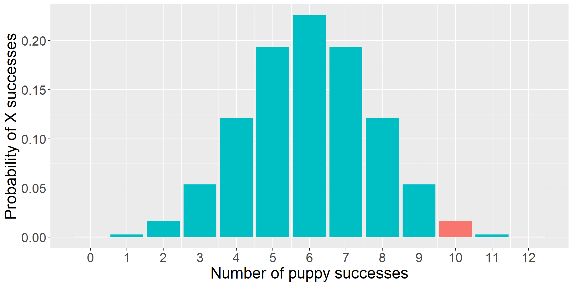
Instead of calculating the probability of our statistic, we calculate the probability of our statistic or more extreme under the null.
The probability of success on 10 trials out of 12 or more extreme is 0.01.
Code
data.frame(trials = trial, d = dbinom(trial, size = 12, prob = .5),
           color = ifelse(trial %in% c(0,1,2, 10,11,12), "1", "2")) %>%
  ggplot(aes(x = trials, y = d, fill = color)) +
  geom_bar(stat = "identity") +
  guides(fill = "none")+
  scale_x_continuous("Number of successes", breaks = c(0:12))+
  scale_y_continuous("Probability of X successes") +
  theme(text = element_text(size = 20))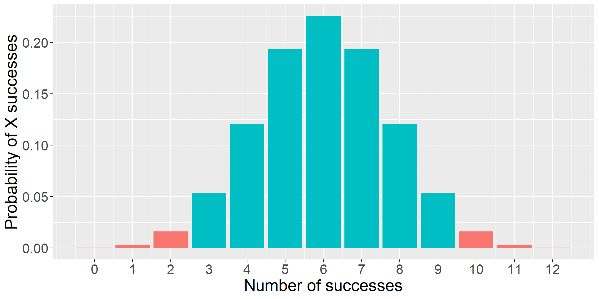
As we have more trials…
Code
data.frame(trials = 0:24,
           d = dbinom(0:24, size = 24, prob = .5),
           color = ifelse(0:24 %in% c(0:4, 20:24), "1", "2")) %>%
  ggplot(aes(x = trials, y = d, fill = color)) +
  geom_bar(stat = "identity") +
  guides(fill = "none")+
  scale_x_continuous("Number of trials hired", breaks = c(0:24))+
  scale_y_continuous("Probability of X trials hired") +
  theme(text = element_text(size = 20))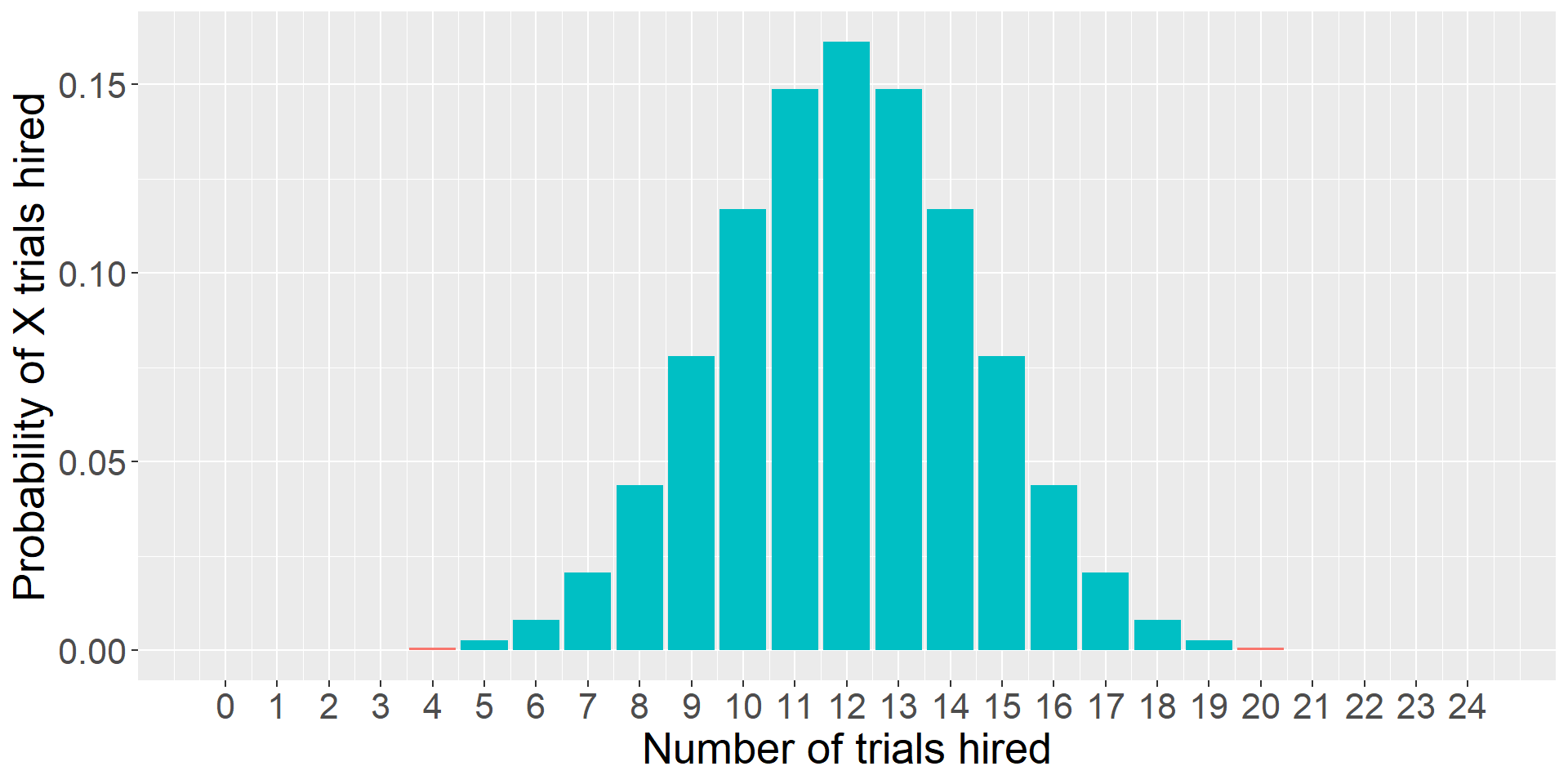
… and more trials…
Code
data.frame(trials = 0:36,
           d = dbinom(0:36, size = 36, prob = .5),
           color = ifelse(0:36 %in% c(0:6, 30:36), "1", "2")) %>%
  ggplot(aes(x = trials, y = d, fill = color)) +
  geom_bar(stat = "identity") +
  guides(fill = "none")+
  scale_x_continuous("Number of trials hired", breaks = c(0:36))+
  scale_y_continuous("Probability of X trials hired") +
  theme(text = element_text(size = 20))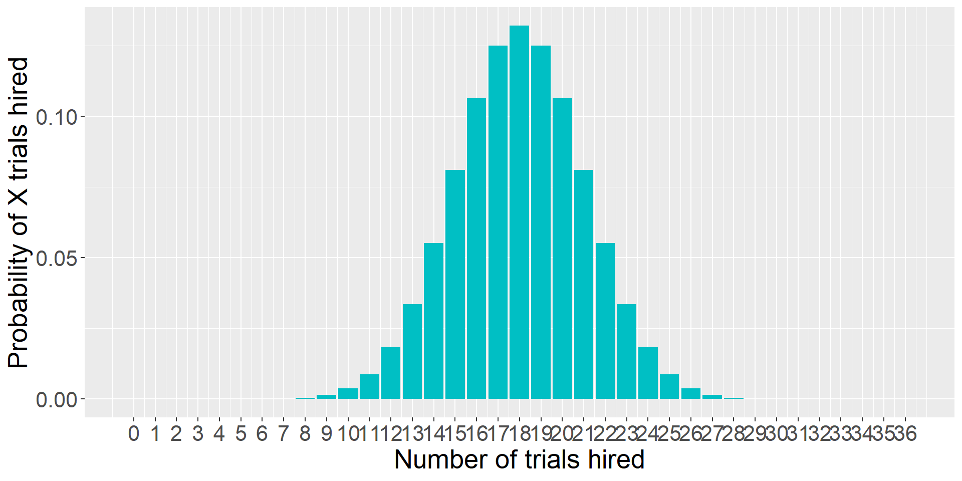
If our measure was continuous, it would look something like this.
Code
gg_color_hue <- function(n) {
  hues = seq(15, 375, length = n + 1)
  hcl(h = hues, l = 65, c = 100)[1:n]
}

colors = gg_color_hue(2)

data.frame(x = seq(-4,4)) %>%
  ggplot(aes(x=x)) +
  stat_function(fun = function(x) dnorm(x), geom = "area", fill = colors[2])+
  stat_function(fun = function(x) dnorm(x), xlim = c(-4, -2.32), geom = "area", fill = colors[1])+
  stat_function(fun = function(x) dnorm(x), xlim = c(2.32, 4), geom = "area", fill = colors[1])+
  geom_hline(aes(yintercept = 0)) +
  scale_x_continuous(breaks = NULL)+
  labs(x = "successes",
       y = "Probability of X successes") +
  theme(text = element_text(size = 20))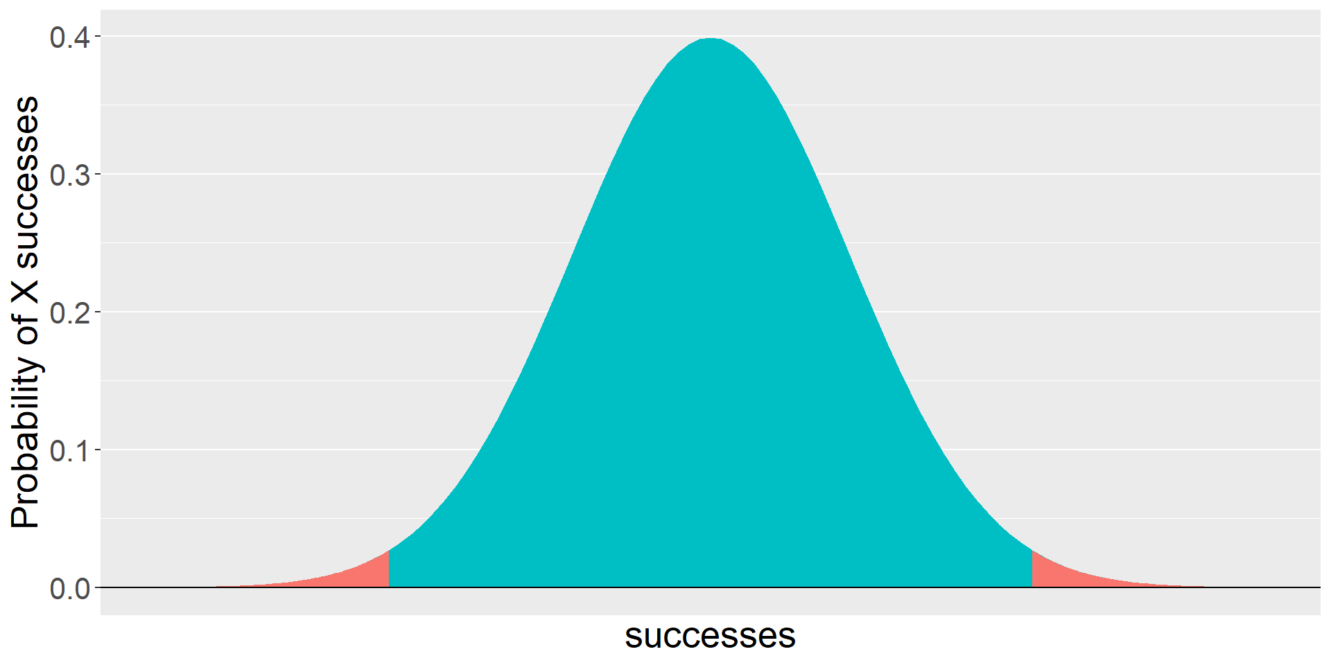
Enter sampling distributions
Code
data.frame(trials = trial, d = dbinom(trial, size = 12, prob = .5),
           color = ifelse(trial %in% c(0,1,2, 10,11,12), "1", "2")) %>%
  ggplot(aes(x = trials, y = d, fill = color)) +
  geom_bar(stat = "identity") +
  guides(fill = "none")+
  scale_x_continuous("Number of successes", breaks = c(0:12))+
  scale_y_continuous("Probability of X successes") +
  theme(text = element_text(size = 20))
When we were analyzing the puppy problem, we built the distribution under the null using the binomial.
This is our sampling distribution.
The mean of the sampling distribution = the mean of the null hypothesis
The standard deviation of the sampling distribution:
\[\small SEM = \frac{\sigma}{\sqrt{N}}\]
Code
data.frame(x = seq(0,100)) %>%
  ggplot(aes(x=x)) +
  stat_function(fun = function(x) dnorm(x, mean = 50, sd = 18.88/sqrt(10)),
                geom = "area", fill = "purple", alpha = .5) +
  stat_function(fun = function(x) dnorm(x, mean = 50, sd = 18.88/sqrt(5)),
                geom = "area", fill = "red", alpha = .5) +
  stat_function(fun = function(x) dnorm(x, mean = 50, sd = 18.88/sqrt(2)),
                geom = "area", fill = "blue", alpha = .5) +
      labs(title = as.expression(bquote("Population"~mu~"=50"~sigma~"=5.97")),
           x = "Average proportion of successes",
           y = NULL)  +
  theme(text = element_text(size = 20))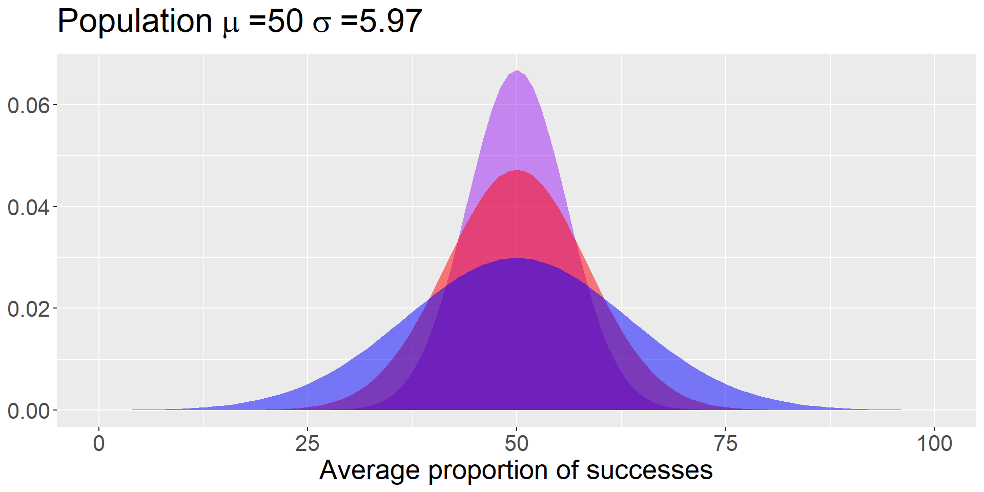
The mean of the sampling distribution = the mean of the null hypothesis
The standard deviation of the sampling distribution:
\[\small SEM = \frac{\sigma}{\sqrt{N}}\]
Code
sem = 18.88/sqrt(10)
data.frame(x = seq(0,100)) %>%
  ggplot(aes(x=x)) +
  stat_function(fun = function(x) dnorm(x, mean = 50, sd = sem),
                geom = "area", alpha = .75) +
      labs(title = as.expression(bquote("Population"~mu~"=50"~sigma~"=5.97")),
           x = "Average proportion of successes",
           y = NULL)  +
  theme(text = element_text(size = 20))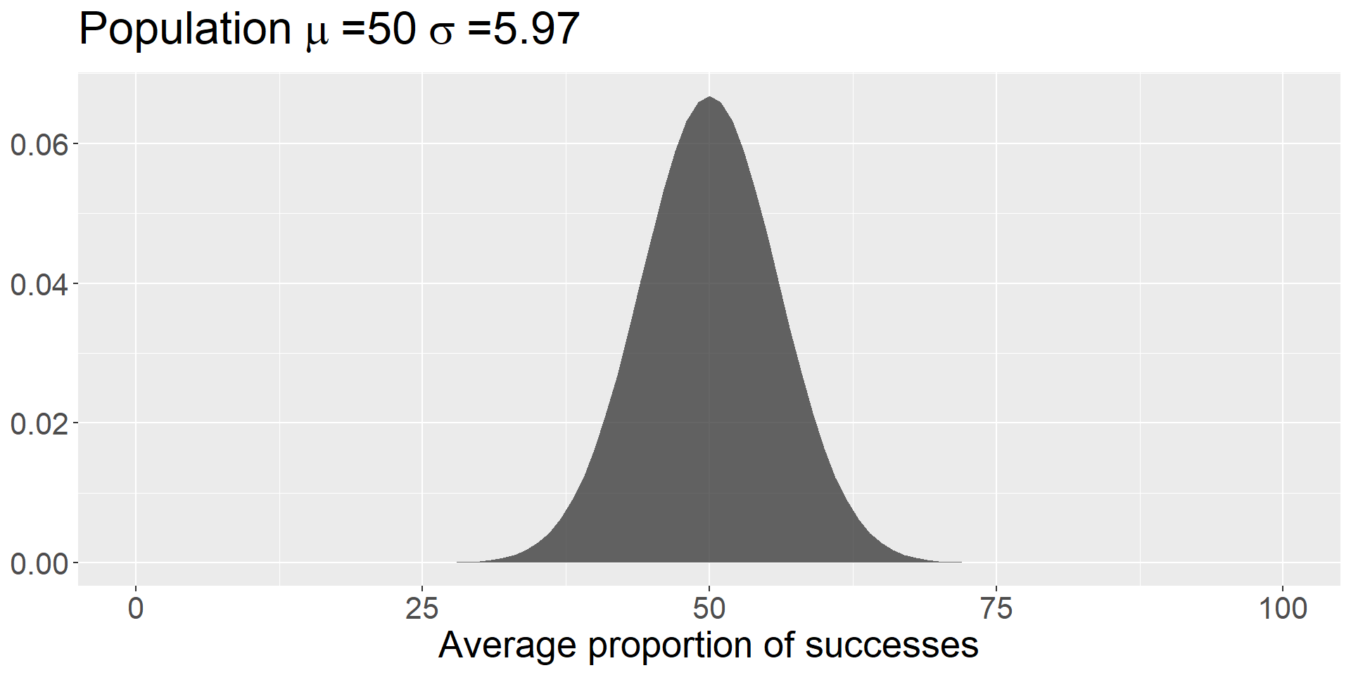
Code
data.frame(x = seq(0,100)) %>%
  ggplot(aes(x=x)) +
  stat_function(fun = function(x) dnorm(x, mean = 50, sd = 18.88/sqrt(10)),
                geom = "area") +
  stat_function(fun = function(x) dnorm(x, mean = 50, sd = 18.88/sqrt(10)),
                geom = "area", xlim = c(0, 35.81), fill = colors[1]) +
  stat_function(fun = function(x) dnorm(x, mean = 50, sd = 18.88/sqrt(10)),
                geom = "area", xlim = c(64.19, 100), fill = colors[1]) +
  geom_vline(aes(xintercept = 64.19), color = "purple") +
      labs(title = as.expression(bquote("Population"~mu~"=50"~sigma~"=5.97")),
           x = "Average proportion of successes",
           y = NULL)  +
  theme(text = element_text(size = 20))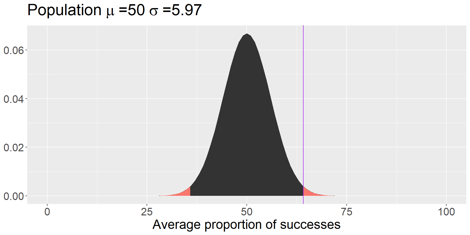
We can use this information to calculate a z-score; in the context of comparing one mean to a sampling distribution of means, we call this a z-statistic.
\[Z = \frac{\bar{X}- M}{SEM} = \frac{69.41-50}{5.97} = 3.25\]
We begin by defining the location in the null hypothesis distribution beyond which empirical results would be considered sufficiently unusual to lead us to reject the null hypothesis. We control these mistakes (Type I errors) at the chosen level of significance ( \(\alpha = .05\) ).
Code
mu = 100
xbar = 110
s = 20
n = 25
sem = s/sqrt(n)
cv = qnorm(mean = mu, sd = sem, p = .025, lower.tail = F)
cv2 = qnorm(mean = mu, sd = sem, p = .025, lower.tail = T)

ggplot(data.frame(x = seq(70, 130)), aes(x)) +
  stat_function(fun = function(x) dnorm(x, m = mu, sd = sem)) +
  stat_function(fun = function(x) dnorm(x, m = mu, sd = sem),
                geom = "area", xlim = c(cv, 130), fill = "red") +
  geom_vline(aes(xintercept = cv), color = "red")+
  stat_function(fun = function(x) dnorm(x, m = mu, sd = sem),
                geom = "area", xlim = c(cv2, 70), fill = "red") +
  geom_vline(aes(xintercept = mu))+
  geom_hline(aes(yintercept = 0))+
  scale_x_continuous("Means", breaks = seq(70,130,10)) +
  scale_y_continuous(NULL, breaks = NULL)+
  theme_pubr() +
  theme(text = element_text(size = 20))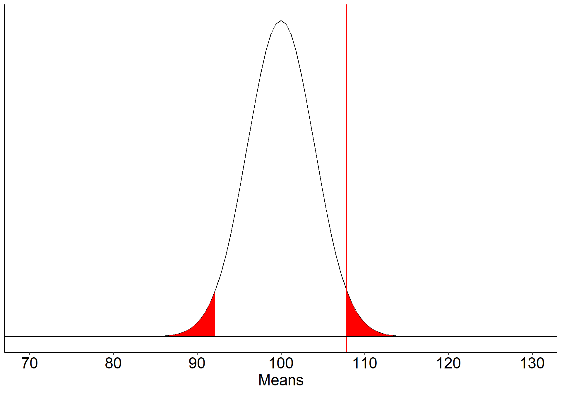
\[\small \text{Critical Value} \\= \mu_0 + Z_{.975}\frac{\sigma}{\sqrt{N}}\\= 100 + 1.96\frac{20}{\sqrt{25}} \\= 107.84\]
What if the null hypothesis is false? How likely are we to correctly reject the null hypothesis in the long run?
Code
mu = 100
xbar = 110
s = 20
n = 25
sem = s/sqrt(n)
cv = qnorm(mean = mu, sd = sem, p = .025, lower.tail = F)
cv2 = qnorm(mean = mu, sd = sem, p = .025, lower.tail = T)

ggplot(data.frame(x = seq(70, 130)), aes(x)) +
  stat_function(fun = function(x) dnorm(x, m = mu, sd = sem)) +
  stat_function(fun = function(x) dnorm(x, m = mu, sd = sem),
                geom = "area", xlim = c(cv, 130), fill = "red") +
  geom_vline(aes(xintercept = cv), color = "red")+
  stat_function(fun = function(x) dnorm(x, m = mu, sd = sem),
                geom = "area", xlim = c(cv2, 70), fill = "red") +
  geom_vline(aes(xintercept = mu))+
  geom_hline(aes(yintercept = 0))+
  scale_x_continuous("Means", breaks = seq(70,130,10)) +
  scale_y_continuous(NULL, breaks = NULL)+
  theme_pubr() +
  theme(text = element_text(size = 20))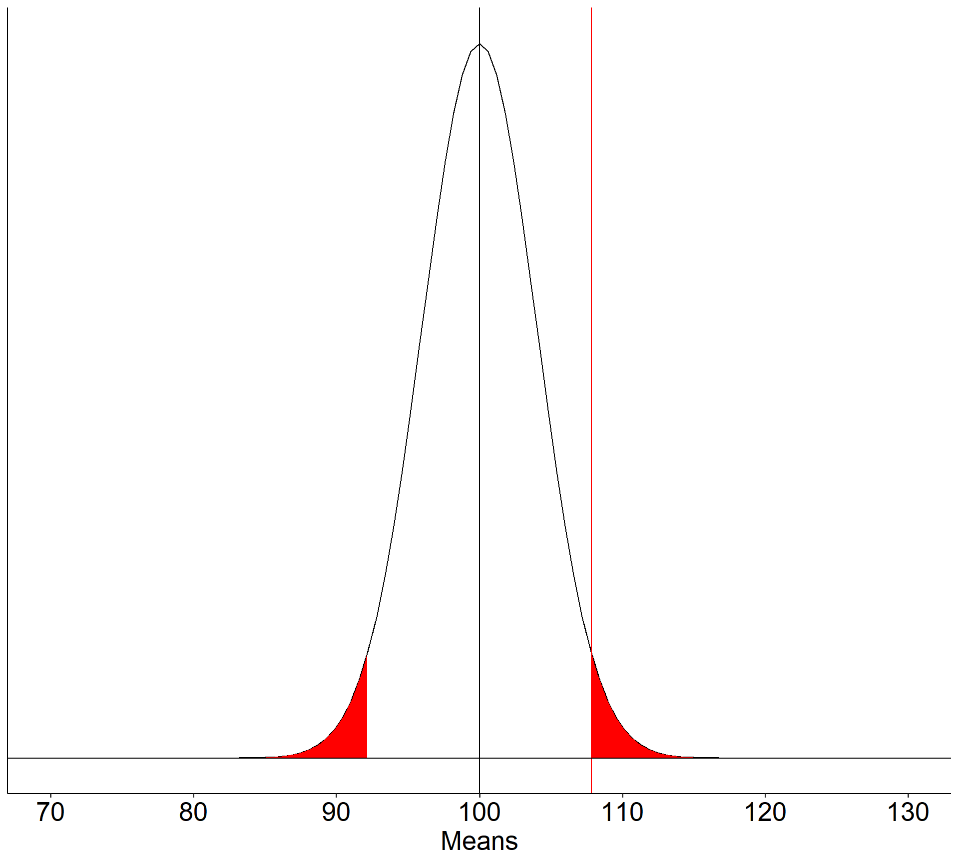
Code
data.frame(x = seq(70, 140)) %>%
  ggplot(aes(x = x)) +
  stat_function(fun = function(x) dnorm(x, mean = mu, sd = sem),
                 geom = "line") +
  stat_function(aes(fill = "Type I error"), fun = function(x) dnorm(x, mean = mu, sd = sem),
                 geom = "area", xlim = c(cv, 140),
                alpha = .5) +
  stat_function(aes(fill = "Type I error"), fun = function(x) dnorm(x, mean = mu, sd = sem),
                 geom = "area", xlim = c(70, cv2),
                alpha = .5) +
  geom_vline(aes(xintercept = cv, color = "Critical Value")) +
  guides(color = "none") +
  scale_x_continuous(limits = c(70,140), breaks = seq(70, 140, 10)) +
  scale_y_continuous(breaks = NULL) +
  labs(x = "Mean", y = "density", fill = NULL)+
  theme_pubr()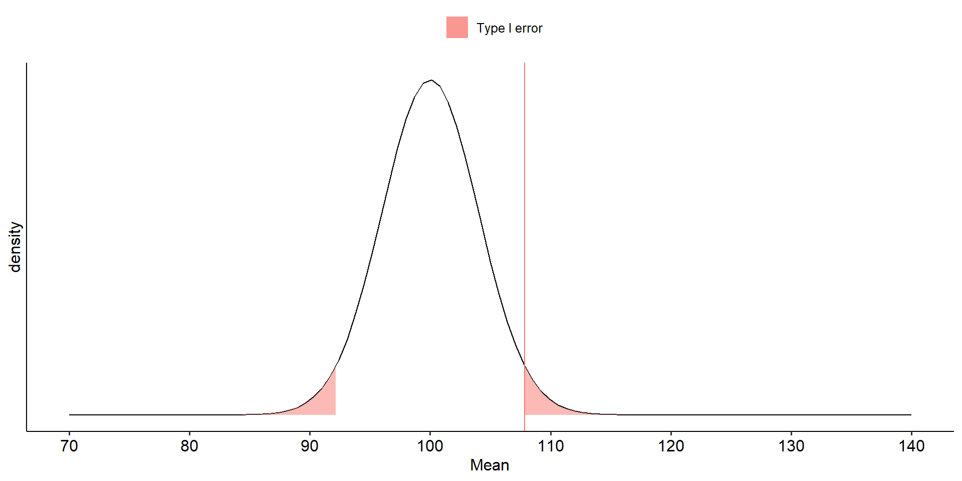
Code
data.frame(x = seq(70, 140)) %>%
  ggplot(aes(x = x)) +
  stat_function(fun = function(x) dnorm(x, mean = mu, sd = sem),
                 geom = "line", alpha = .2) +
  geom_vline(aes(xintercept = cv, color = "Critical Value")) +
  guides(color = "none") +
  scale_x_continuous(limits = c(70,140), breaks = seq(70, 140, 10)) +
  scale_y_continuous(breaks = NULL) +
  labs(x = "Mean", y = "density", fill = NULL)+
  theme_pubr()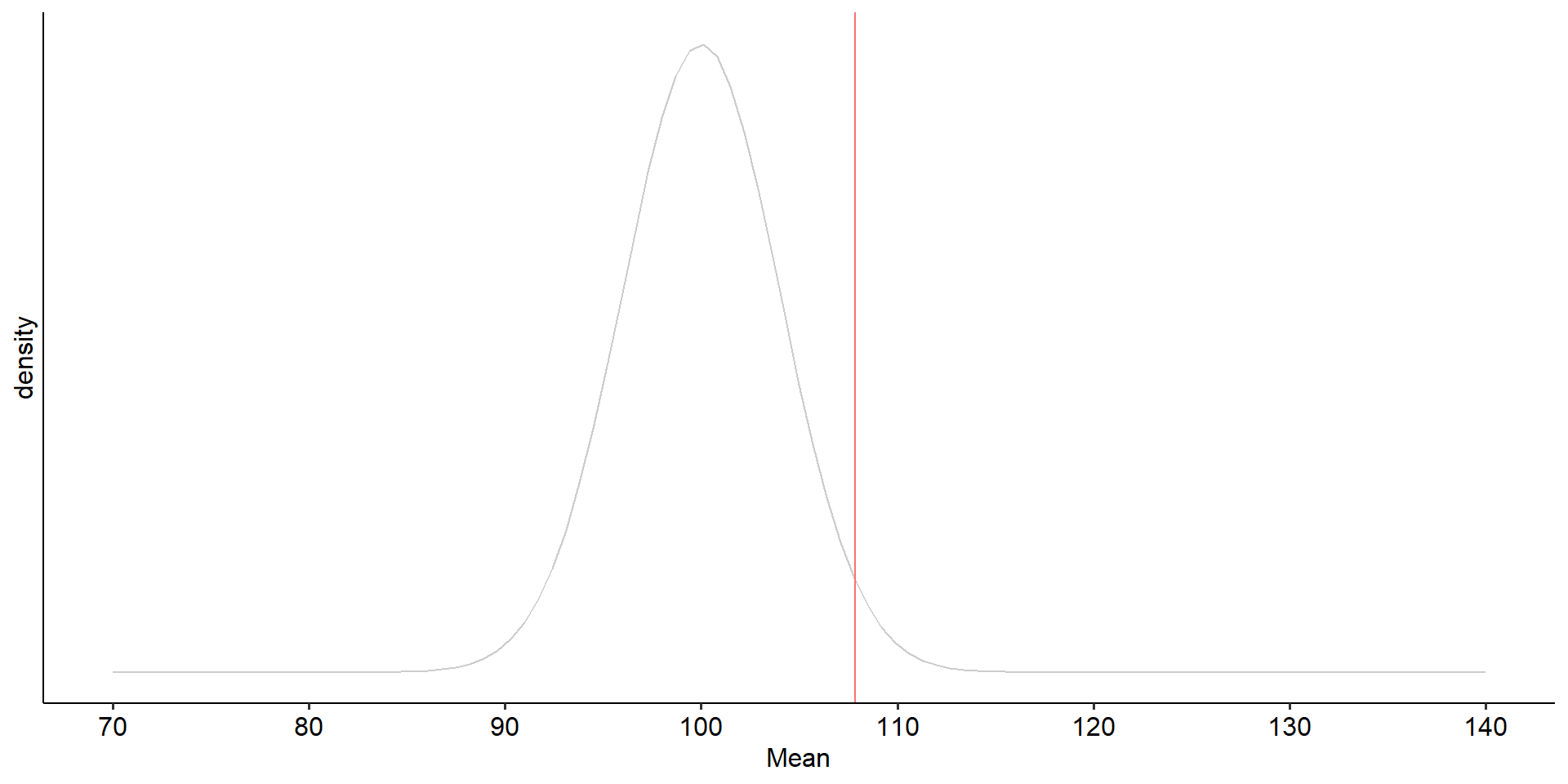
Code
data.frame(x = seq(70, 140)) %>%
  ggplot(aes(x = x)) +
  stat_function(fun = function(x) dnorm(x, mean = mu, sd = sem),
                 geom = "line", alpha = .2) +
  stat_function(fun = function(x) dnorm(x, mean = xbar, sd = sem),
                 geom = "line") +
  geom_vline(aes(xintercept = cv, color = "Critical Value")) +
  guides(color = "none") +
  scale_x_continuous(limits = c(70,140), breaks = seq(70, 140, 10)) +
  scale_y_continuous(breaks = NULL) +
  labs(x = "Mean", y = "density", fill = NULL)+
  theme_pubr()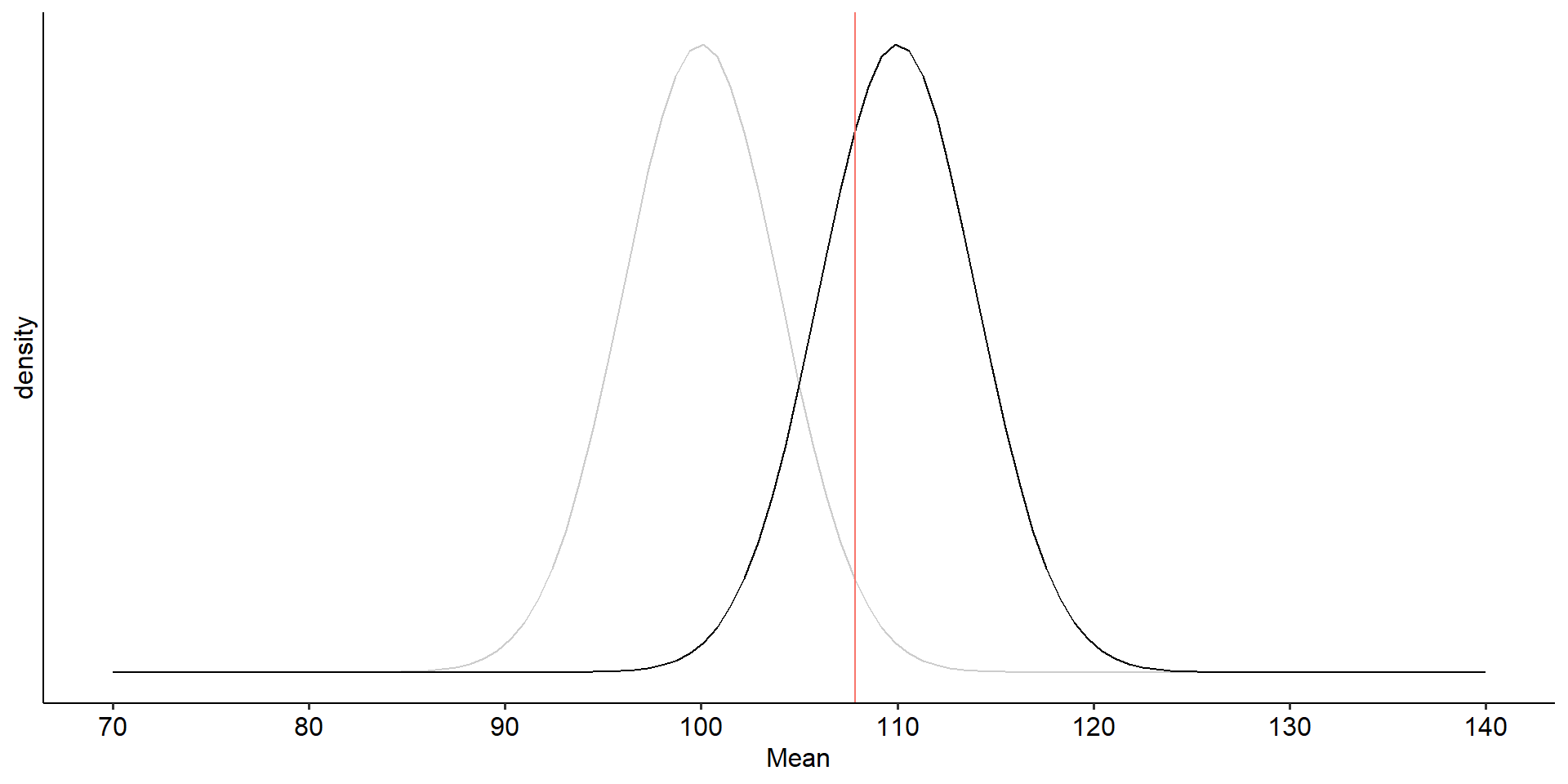
Code
data.frame(x = seq(70, 140)) %>%
  ggplot(aes(x = x)) +
  stat_function(fun = function(x) dnorm(x, mean = mu, sd = sem),
                 geom = "line", alpha = .2) +
  stat_function(fun = function(x) dnorm(x, mean = xbar, sd = sem),
                 geom = "line") +
  stat_function(aes(fill = "Power"), fun = function(x) dnorm(x, mean = xbar, sd = sem),
                 geom = "area", xlim = c(cv, 140),
                alpha = .5) +
  stat_function(aes(fill = "Type II error"), fun = function(x) dnorm(x, mean = xbar, sd = sem),
                 geom = "area", xlim = c(70, cv),
                alpha = .5) +
  geom_vline(aes(xintercept = cv, color = "Critical Value")) +
  guides(color = "none") +
  scale_x_continuous(limits = c(70,140), breaks = seq(70, 140, 10)) +
  scale_y_continuous(breaks = NULL) +
  labs(x = "Mean", y = "density", fill = NULL)+
  theme_pubr()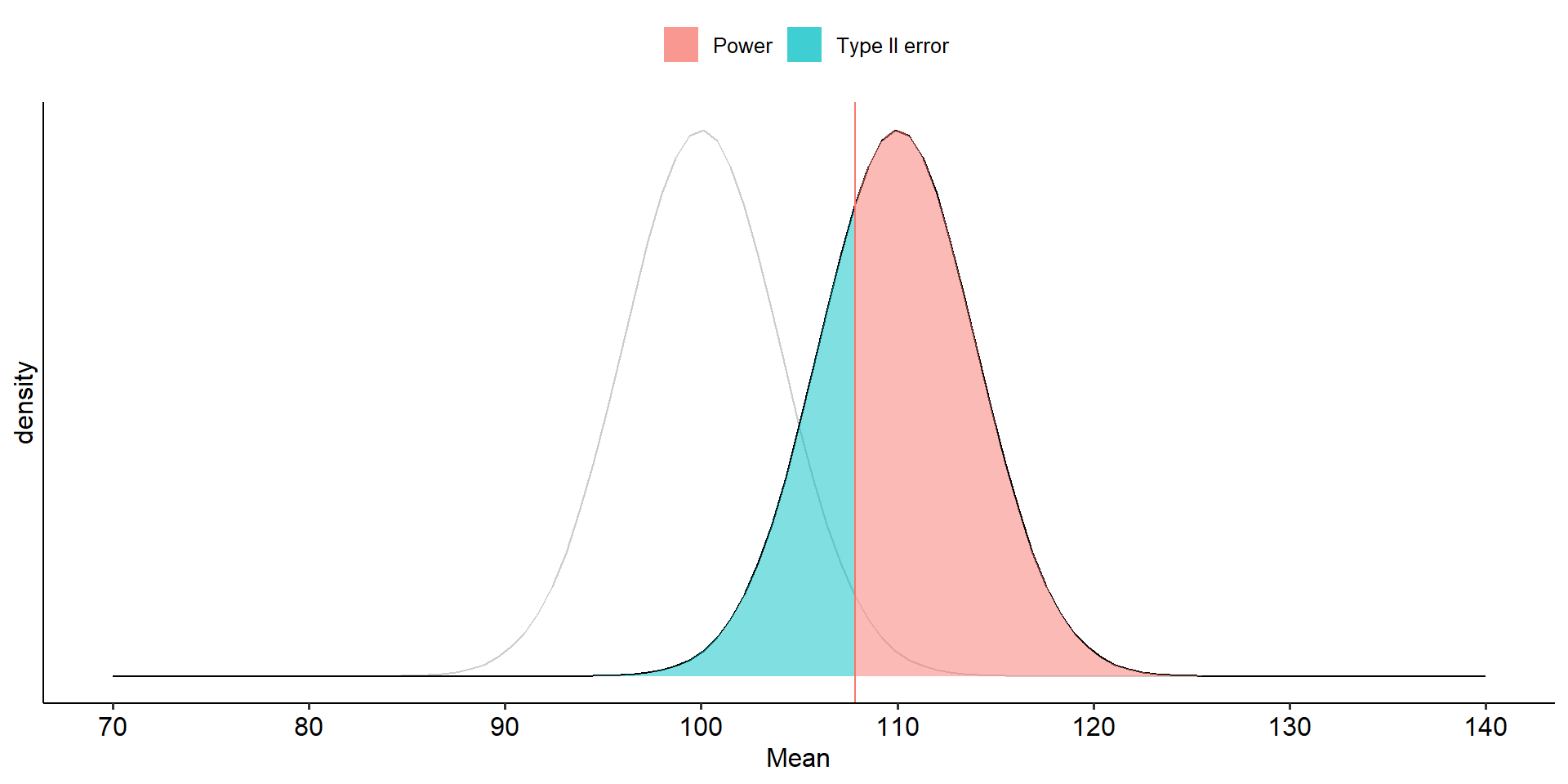
To determine the probability of a Type II error, we must specify a value for the alternative hypothesis. We will use the sample mean of 110.
In the long run, if psychology samples have a mean of 110 ( \(\sigma = 20\), \(N = 25\) ), we will correctly reject the null with probability of 0.71 (power). We will incorrectly fail to reject the null with probability of 0.29 ( \(\beta\) ).
Another way to determine these values: Once the critical value and alternative value is established, we can determine the location of the critical value in the alternative distribution.
[1] -0.540036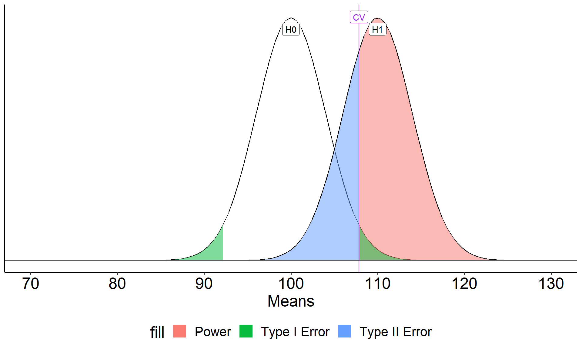
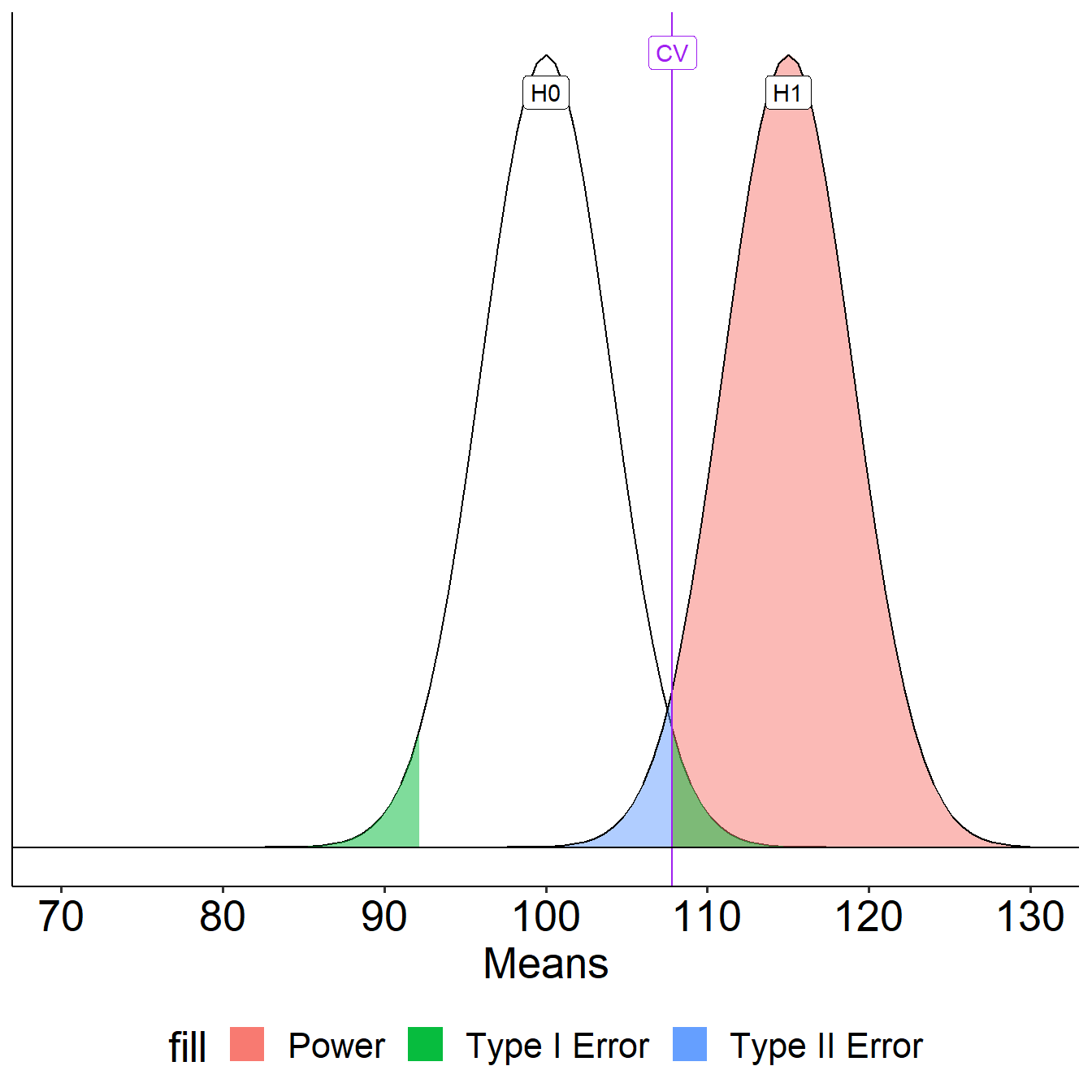
Changing Effect Size
The choice of 110 as the mean of \(H_1\) is completely arbitrary. What if we believe that the alternative mean is 115? This larger signal should be easier to detect.
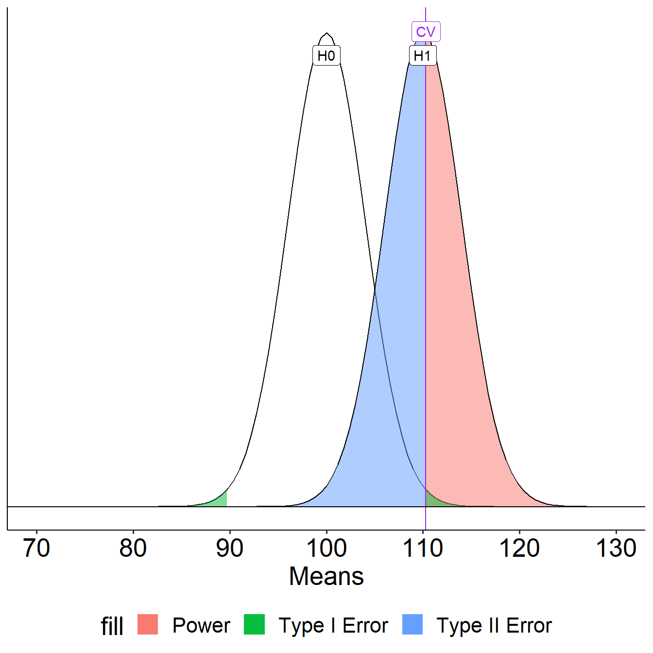
Increase Sample Size
What if instead we increase the sample size? This will reduce variability in the sampling distribution, making the difference between the null and alternative distributions easier to see. (New \(N\) is 50.)

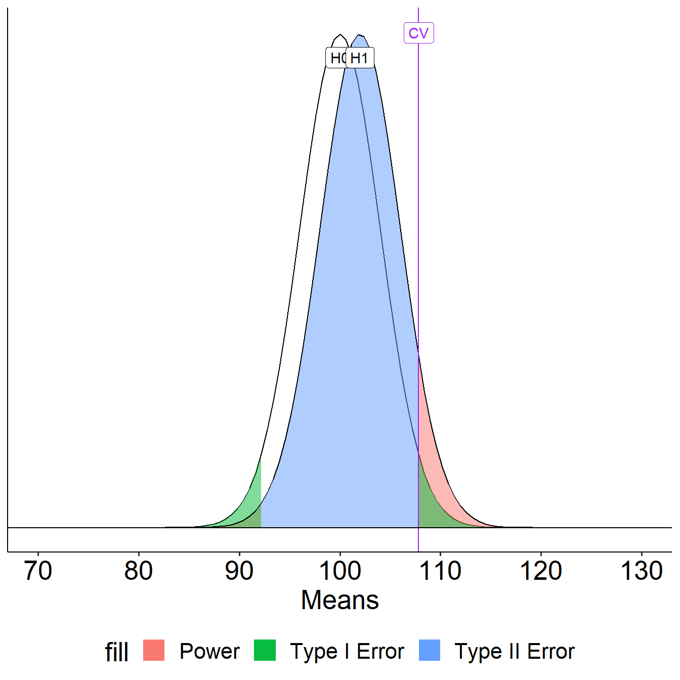
Update \(\alpha\)
What if we decrease the significance level to .01?
Oops, we’ve been ignoring the other tail. So far it hasn’t mattered (the area has been so small) but it makes a difference when \(H_0\) and \(H_1\) overlap significantly.
More generally we can determine the relationship between effect size and power for a constant \(\alpha\) (.05) and sample size ( \(N = 20\) ).
Code
pwr_fun = function(m1, m2, alpha, n, sd){
  sem = sd/sqrt(n)
  cv = qnorm(p = 1-(alpha/2), mean = m1, sd = sem)
  z_1 = (cv-m2)/sem
  power = pnorm(q = z_1, lower.tail = F)
  return(power)
}

size = seq(100, 120, 1)

data.frame(effect = size, power = sapply(size, function(x) pwr_fun(m1 = 100, m2 = x, alpha = .05, n = 20, sd = 20))) %>%
  ggplot(aes(x = effect, y = power)) +
  geom_line(size = 1.5) +
  scale_x_continuous(expression(H[1]~Mean)) +
  ggtitle("Power to detect significant effect by mean") +
  theme_pubr() +
  theme(text = element_text(size = 20))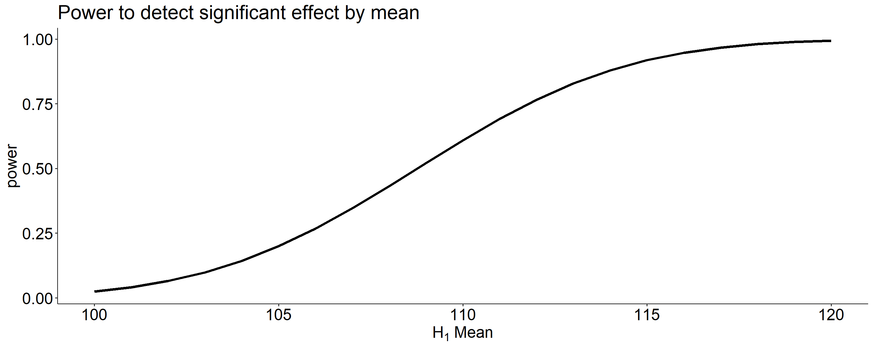
Likewise, we can display the relationship between sample size and power for a constant \(\alpha\) and effect size.
Below is difference of means 100 to 110 in our example
Code
size = seq(5,200,5)

data.frame(size = size, power = sapply(size, function(x) pwr_fun(m1 = 100, m2 = 110, alpha = .05, n = x, sd = 20))) %>%
  ggplot(aes(x = size, y = power)) +
  geom_line(size = 1.5) +
  scale_x_continuous("Sample Size") +
  ggtitle("Power to detect significant effect by sample size") +
  theme_pubr() +
  theme(text = element_text(size = 20))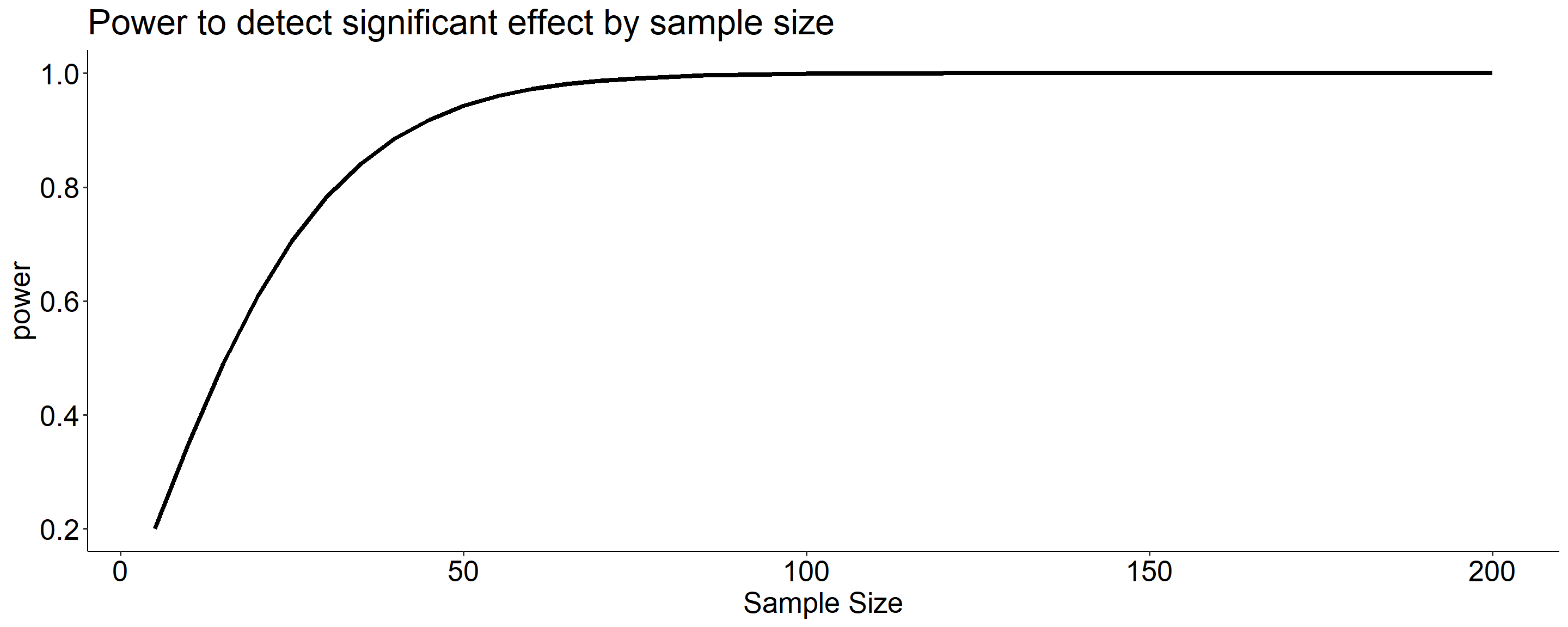
Power changes as a function of significance level for a constant effect size and sample size.
Code
size = seq(.01,.20,.01)

data.frame(alpha = size,
           power = sapply(size, function(x) pwr_fun(m1 = 100,
                                                    m2 = 110,
                                                    alpha = x,
                                                    n = 20,
                                                    sd = 20))) %>%
  ggplot(aes(x = alpha, y = power)) +
  geom_line(size = 1.5) +
  scale_x_continuous(expression(alpha)) +
  ggtitle("Power to detect significant effect by alpha") +
  theme_pubr() +
  theme(text = element_text(size = 20))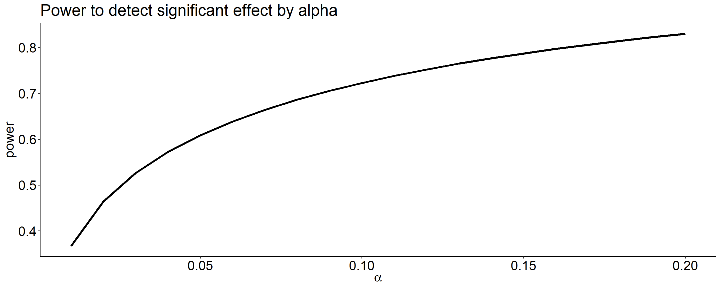
For a one-tailed test, we put the entire rejection area into a single tail. If \(\alpha = .05\), then one tail contains .05 and critical values will be either 1.64 or -1.64 standard errors away from the null mean.
Code
mu = 100
x = 110
s = 20
n = 25
sem = s/sqrt(n)
cv_sngle = qnorm(mean = mu, sd = sem, p = .05, lower.tail = F)

ggplot(data.frame(x = seq(70, 130)), aes(x)) +
  stat_function(fun = function(x) dnorm(x, m = mu, sd = sem)) +
  stat_function(fun = function(x) dnorm(x, m = mu, sd = sem),
                geom = "area", xlim = c(cv_sngle, 130), fill = "red") +
  geom_vline(aes(xintercept = cv_sngle), color = "red")+
  geom_vline(aes(xintercept = mu))+
  geom_hline(aes(yintercept = 0))+
  scale_x_continuous("Means", breaks = seq(70,130,10)) +
  scale_y_continuous(NULL, breaks = NULL) +
  theme_pubr() +
  theme(text = element_text(size = 20))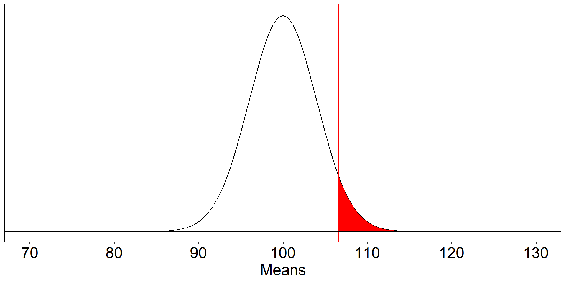
A two-tailed test is less powerful (more conservative) than a one-tailed test for the same sample size.
Code
pwr1_fun = function(m1, m2, alpha, n, sd){
  sem = sd/sqrt(n)
  cv = qnorm(p = 1-(alpha), mean = m1, sd = sem)
  z_1 = (cv-m2)/sem
  power = pnorm(q = z_1, lower.tail = F)
  return(power)
}
pwr2_fun = function(m1, m2, alpha, n, sd){
  sem = sd/sqrt(n)
  cv_1 = qnorm(p = 1-(alpha/2), mean = m1, sd = sem)
  cv_2 = qnorm(p = (alpha/2), mean = m1, sd = sem)
  z_1 = (cv_1-m2)/sem
  z_2 = (cv_2-m2)/sem
  power = pnorm(q = z_1, lower.tail = F) + pnorm(q = z_2, lower.tail = T)
  return(power)
}

size = seq(5,100,5)

data.frame(effect = size,
           power_1 = sapply(size, function(x) pwr1_fun(m1 = 100, m2 = 110, alpha = .05, n = x, sd = 20)),
           power_2 = sapply(size, function(x) pwr2_fun(m1 = 100, m2 = 110, alpha = .05, n = x, sd = 20))) %>%
  ggplot(aes(x = effect)) +
  geom_line(aes(y = power_1, color = "one-tail"), size = 1.5) +
  geom_line(aes(y = power_2, color = "two-tail"), size = 1.5) +
  scale_x_continuous("Sample Size") +
  scale_y_continuous("power")+
  ggtitle("Power to detect significant effect by mean") +
  theme_pubr() +
  theme(text = element_text(size = 20))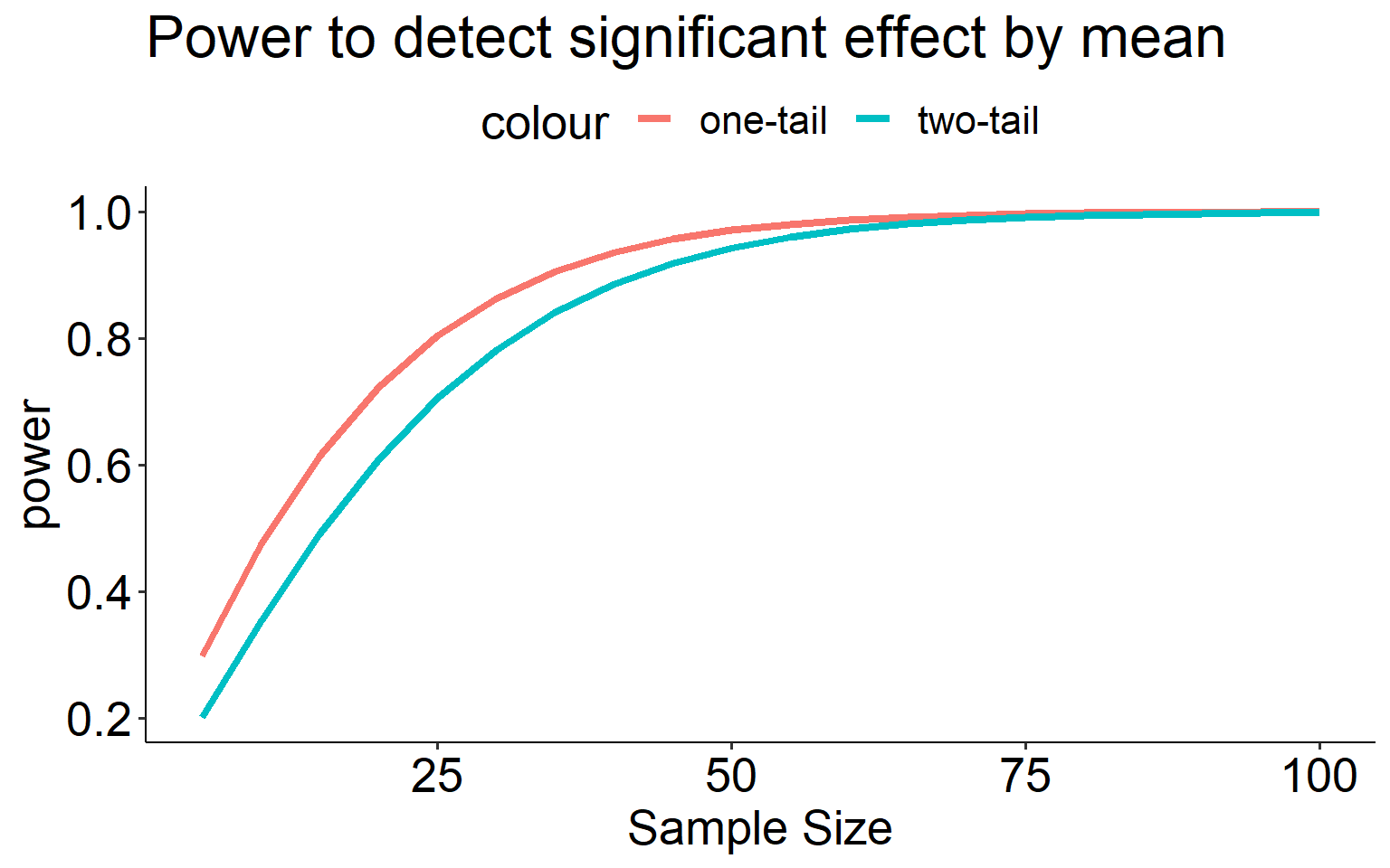
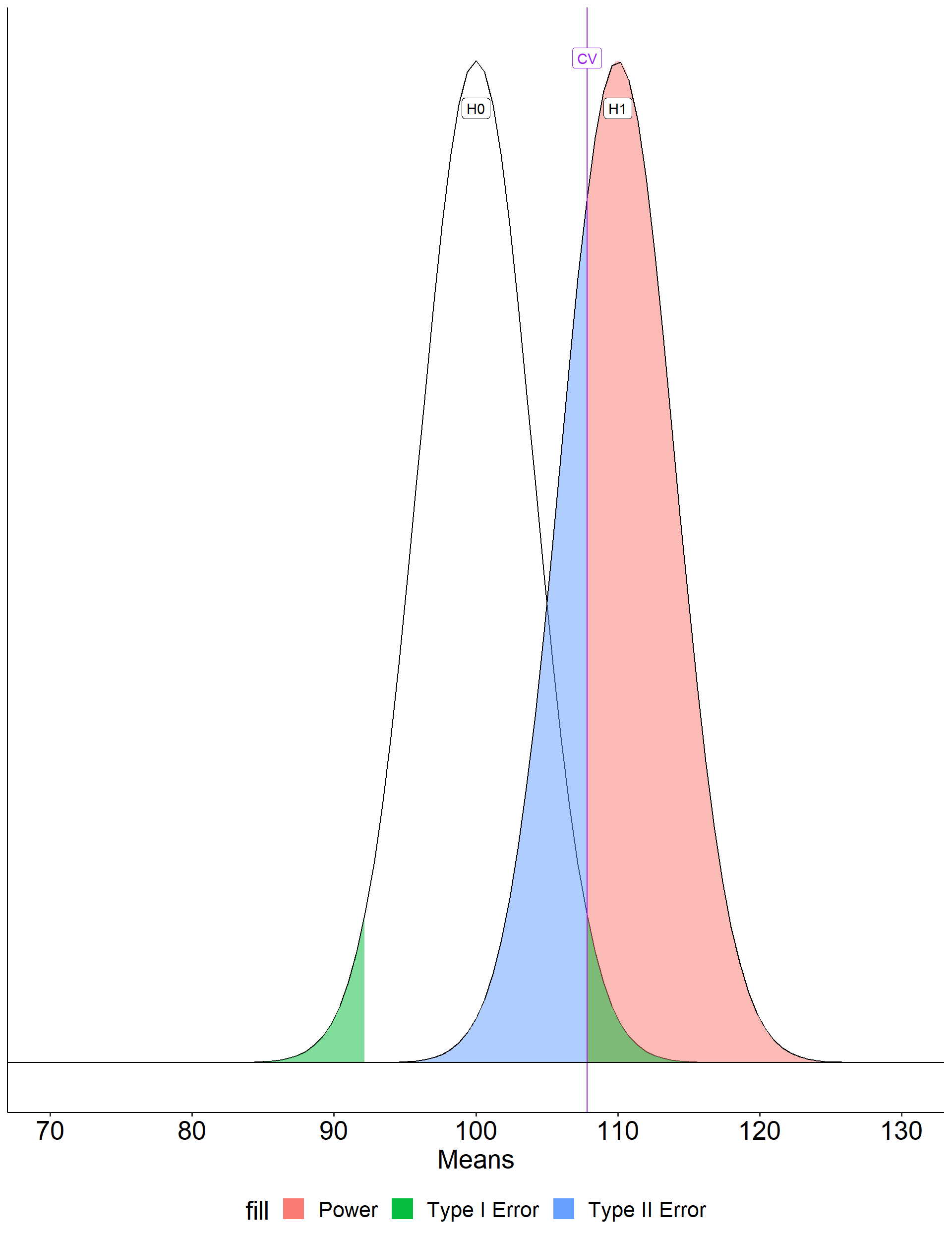
How can power be increased?
Code
#|
ggplot(data.frame(x = seq(70, 130)), aes(x)) +
  stat_function(fun = function(x) dnorm(x, m = mu, sd = sem)) +

  stat_function(fun = function(x) dnorm(x, m = mean, sd = sem),
                geom = "area", xlim = c(cv, 130),
                aes(fill = "Power"), alpha = .5) +
  stat_function(fun = function(x) dnorm(x, m = mean, sd = sem),
                geom = "area", xlim = c(70, cv2),
                aes(fill = "Power"), alpha = .5) +
  stat_function(fun = function(x) dnorm(x, m = mean, sd = sem),
                geom = "area", xlim = c(cv2, cv),
                aes(fill = "Type II Error"), alpha = .5) +
  stat_function(fun = function(x) dnorm(x, m = mu, sd = sem),
                geom = "area", xlim = c(cv, 130),
                aes(fill = "Type I Error"), alpha = .5) +
  stat_function(fun = function(x) dnorm(x, m = mu, sd = sem),
                geom = "area", xlim = c(cv2, 70),
                aes(fill = "Type I Error"), alpha = .5) +
  stat_function(fun = function(x) dnorm(x, m = mean, sd = sem)) +
  geom_vline(aes(xintercept = cv), color = "purple")+
  geom_label(aes(x = mu, y = .095, label = "H0")) +
  geom_label(aes(x = mean, y = .095, label = "H1")) +
  geom_label(aes(x = cv, y = .1, label = "CV"), color = "purple") +
  geom_hline(aes(yintercept = 0))+
  scale_x_continuous("Means", breaks = seq(70,130,10)) +
  scale_y_continuous(NULL, breaks = NULL) +
  theme_pubr() +
  theme( text = element_text(size = 20),
    legend.position = "bottom")
\[Z_1 = \frac{CV_0 - \mu_1}{\frac{\sigma}{\sqrt{N}}}\]
- increase \(\mu_1\)
- decrease \(CV_0\)
- increase \(N\)
- reduce \(\sigma\)
I strongly recommend playing around with different configurations of \(N\), \(\alpha\) and the difference in means ( \(d\) ) in this online demo.