Categorical Data & Comparing Means
PSYC 640 - Fall 2023
Last week
- Review of the NHST
- Categorical Data analysis with the \(\chi^2\) distribution
- Goodness of Fit test
Today…
- The chi-square test of independence (Book Chapter 12.2)
- Review Assumptions of chi-square test
- Introduction to Comparing Means
Pop Quiz…jk
What do we mean when we say a study was powered to an effect of 0.34?
What does a p-value tell us?
\(\chi^2\) test of independence or association
The previous tests that we conducted last class, we were focused on the way our data (NY Students Superpower Preferences) “fit” to the data of an expected distribution (US Student Superpower Preferences)
Although this could be interesting, sometimes we have two categorical variables that we want to compare to one another
- How do types of traffic stops differ by the gender identity of the police officer?
Let’s take a look at a scenario:
We are part of a delivery company called Planet Express

Let’s take a look at a scenario:
We are part of a delivery company called Planet Express
We have been tasked to deliver a package to Chapek 9

Let’s take a look at a scenario:
We are part of a delivery company called Planet Express
We have been tasked to deliver a package to Chapek 9
Unfortunately, the planet is inhabited completely by robots and humans are not allowed
In order to deliver the package, we have to go through the guard gate and prove that we are able to gain access
At the guard gate
(Robot Voice)
WHICH OF THE FOLLOWING WOULD YOU MOST PREFER?
A: A Puppy
B: A pretty flower from your sweetie
C: A large properly-formatted data file
CHOOSE NOW!
- Clearly an ingenious test that will catch any imposters!
- But what if humans and robots have similar preferences?
Luckily, I have connections with Chapek 9 and we can see if there are any similarities between the responses.
Let’s work through how to do a \(\chi^2\) test of independence (or association)
First, we have to load in the data:
Chapek 9 Data
Take a peek at the data:
Chapek 9 Data
Look at the summary stats for the data:
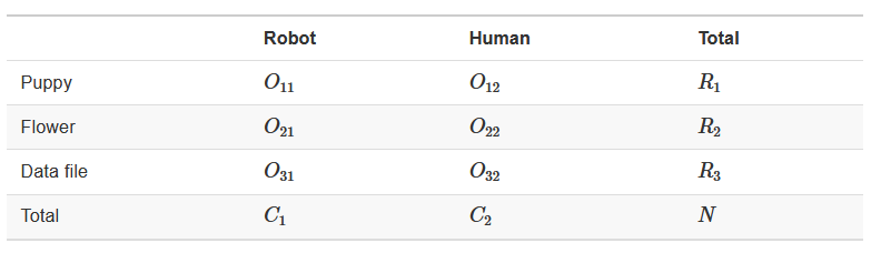
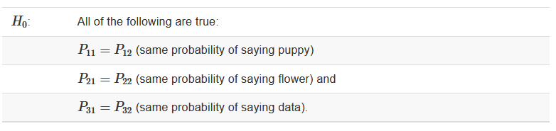
Chapek 9 Data - Cross Tabs
There are a few different ways to look at these tables. We can use xtabs()
Constructing Hypotheses
Research hypothesis states that “humans and robots answer the question in different ways”
Now our notation has two subscript values?? What torture is this??
Constructing Hypotheses
Once we have this established, we can take a look at the null
Claiming now that the true choice probabilities don’t depend on the species making the choice ( \(P_i\) )
However, we don’t know what the expected probability would be for each answer choice
- We have to calculate the totals of each row/column
Chapek 9 Data - Cross Tabs
Let’s use R to make the table look fancy and calculate the totals for us!
We will use the library sjPlot (link)
Note: Will need to knit the document to get this table
| choice | species | Total | |
|---|---|---|---|
| human | robot | ||
| data | 65 | 44 | 109 |
| flower | 13 | 30 | 43 |
| puppy | 15 | 13 | 28 |
| Total | 93 | 87 | 180 |
| χ2=10.722 · df=2 · Cramer's V=0.244 · p=0.005 | |||
Note about degrees of freedom
Degrees of freedom comes from the number of data points that you have, minus the number of constraints
Using contingency tables (or cross-tabs), the data points we have are \(rows * columns\)
There will be two constraints and \(df = (rows-1) * (columns-1)\)
We now have all the pieces for a \(classic\) Null Hypothesis Significance Test
But we have these computers, so why not use them?
Using the associationTest() from the lsr library
Chi-square test of categorical association
Variables: choice, species
Hypotheses:
null: variables are independent of one another
alternative: some contingency exists between variables
Observed contingency table:
        species
choice   human robot
  data      65    44
  flower    13    30
  puppy     15    13
Expected contingency table under the null hypothesis:
species
choice human robot
data 56.3 52.7
flower 22.2 20.8
puppy 14.5 13.5
Test results:
X-squared statistic: 10.722
degrees of freedom: 2
p-value: 0.005
Other information:
estimated effect size (Cramer's v): 0.244 Maybe we want to keep it traditional and use chisq.test() will there be a difference?
Book Ch 12.6 - The most typical way to do a chi-square test in R
But what if we want to visualize it? Use sjPlot again
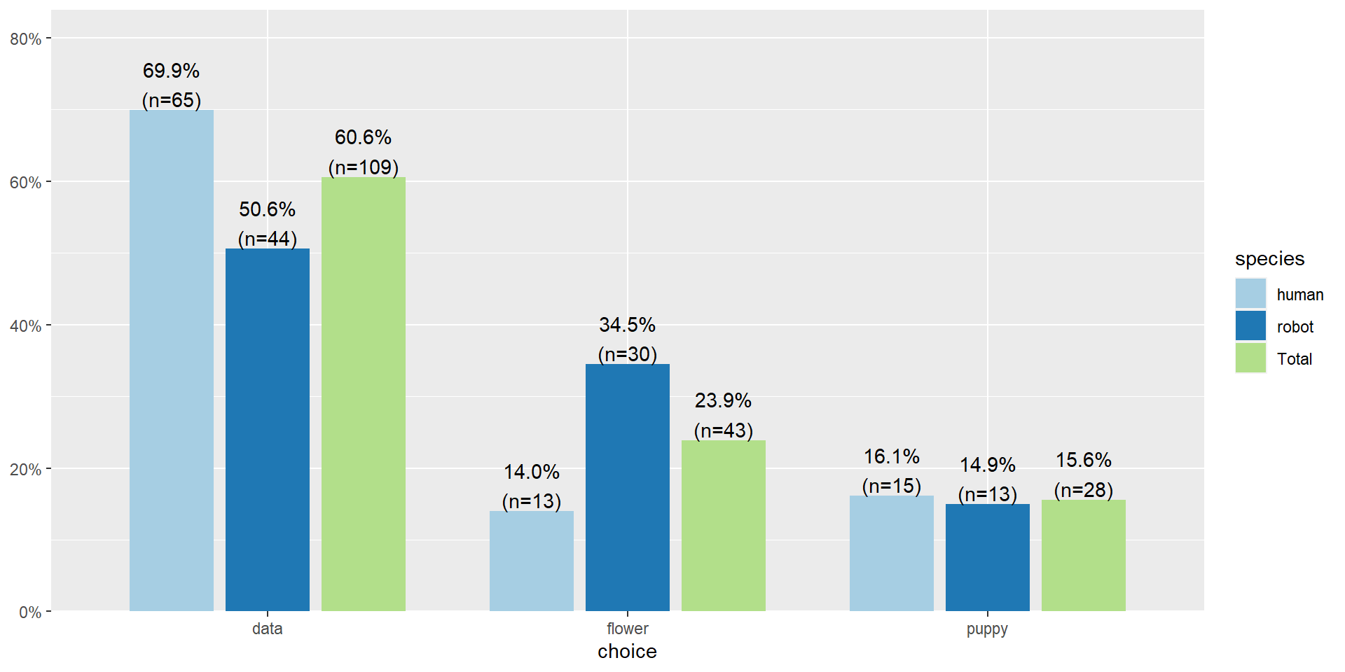
Let’s clean that up a little bit more
Writing it up
Pearson's \(\chi^2\) revealed a significant association between species and choice ( \(\chi^2 (2) =\) 10.7, \(p\) < .01), such that robots appeared to be more likely to say that they prefer flowers, but the humans were more likely to say they prefer data.
Assumptions of the test
The expected frequencies are rather large
Data are independent of one another
Comparing Means
When we move from categorical outcomes to variables measured on an interval or ratio scale, we become interested in means rather than frequencies. Comparing means is usually done with the t-test, of which there are several forms.
The one-sample t-test is appropriate when a single sample mean is compared to a population mean but the population standard deviation is unknown. A sample estimate of the population standard deviation is used instead. The appropriate sampling distribution is the t-distribution, with N-1 degrees of freedom.
\[t_{df=N-1} = \frac{\bar{X}-\mu}{\frac{\hat{\sigma}}{\sqrt{N}}}\]
The heavier tails of the t-distribution, especially for small N, are the penalty we pay for having to estimate the population standard deviation from the sample.
One-sample t-tests
t-tests were developed by William Sealy Gosset, who was a chemist studying the grains used in making beer. (He worked for Guinness.)
Specifically, he wanted to know whether particular strains of grain made better or worse beer than the standard.
He developed the t-test, to test small samples of beer against a population with an unknown standard deviation.
- Probably had input from Karl Pearson and Ronald Fisher
Published this as “Student” because Guinness didn’t want these tests tied to the production of beer.
Load in the dataset from last class
One-sample t-tests vs Z-test
| Z-test | t-test | |
|---|---|---|
| \(\large{\mu}\) | known | known |
| \(\sigma\) | known | unknown |
| sem or \(\sigma_M\) | \(\frac{\sigma}{\sqrt{N}}\) | \(\frac{\hat{\sigma}}{\sqrt{N}}\) |
| Probability distribution | standard normal | \(t\) |
| DF | none | \(N-1\) |
| Tails | One or two | One or two |
| Critical value \((\alpha = .05, two-tailed)\) | 1.96 | Depends on DF |
Assumptions of the one-sample t-test
Normality. We assume the sampling distribution of the mean is normally distributed. Under what two conditions can we be assured that this is true?
Independence. Observations in the dataset are not associated with one another. Put another way, collecting a score from Participant A doesn’t tell me anything about what Participant B will say. How can we be safe in this assumption?
A brief example
Using the same Census at School data, we find that New York students who participated in a memory game ( \(N = 224\) ) completed the game in an average time of 44.2 seconds ( \(s = 15.3\) ). We know that the average US student completed the game in 45.04 seconds. How do our students compare?
Hypotheses
\(H_0: \mu = 45.05\)
\(H_1: \mu \neq 45.05\)
\[\mu = 45.05\]
\[N = 227\]
\[ \bar{X} = 44.2 \]
\[ s = 15.3 \]
    One Sample t-test

data:  school$Score_in_memory_game
t = -0.86545, df = 223, p-value = 0.3877
alternative hypothesis: true mean is not equal to 45.05
95 percent confidence interval:
 42.14729 46.18116
sample estimates:
mean of x
 44.16422
   One sample t-test

Data variable:   school$Score_in_memory_game

Descriptive statistics:
            Score_in_memory_game
   mean                   44.164
   std dev.               15.318

Hypotheses:
   null:        population mean equals 45.05
   alternative: population mean not equal to 45.05

Test results:
   t-statistic:  -0.865
   degrees of freedom:  223
   p-value:  0.388

Other information:
   two-sided 95% confidence interval:  [42.147, 46.181]
   estimated effect size (Cohen's d):  0.058
Cohen’s D
Cohen suggested one of the most common effect size estimates—the standardized mean difference—useful when comparing a group mean to a population mean or two group means to each other.
\[\delta = \frac{\mu_1 - \mu_0}{\sigma} \approx d = \frac{\bar{X}-\mu}{\hat{\sigma}}\]
Cohen’s d is in the standard deviation (Z) metric.
Cohens’s d for these data is .05. In other words, the sample mean differs from the population mean by .05 standard deviation units.
Cohen (1988) suggests the following guidelines for interpreting the size of d:
.2 = Small
.5 = Medium
.8 = Large
Cohen, J. (1988), Statistical power analysis for the behavioral sciences (2nd Ed.). Hillsdale: Lawrence Erlbaum.
The usefulness of the one-sample t-test
How often will you conducted a one-sample t-test on raw data?
- (Probably) never
How often will you come across one-sample t-tests?
- (Probably) a lot!
The one-sample t-test is used to test coefficients in a model.
#Load sleep data: https://vincentarelbundock.github.io/Rdatasets/datasets.html
sleep <- read_csv("https://raw.githubusercontent.com/dharaden/dharaden.github.io/main/data/sleepstudy.csv")
model = lm(Reaction ~ Days, data = sleep)
summary(model)
Call:
lm(formula = Reaction ~ Days, data = sleep)

Residuals:
     Min       1Q   Median       3Q      Max
-110.848  -27.483    1.546   26.142  139.953

Coefficients:
            Estimate Std. Error t value Pr(>|t|)
(Intercept)  251.405      6.610  38.033  < 2e-16 ***
Days          10.467      1.238   8.454 9.89e-15 ***
---
Signif. codes:  0 '***' 0.001 '**' 0.01 '*' 0.05 '.' 0.1 ' ' 1

Residual standard error: 47.71 on 178 degrees of freedom
Multiple R-squared:  0.2865,    Adjusted R-squared:  0.2825
F-statistic: 71.46 on 1 and 178 DF,  p-value: 9.894e-15
Next time…
More comparing means!
Reminders
No Class 10/9
No Office Hours tomorrow (10/5)
Next lab will likely begin on 10/16