Comparing Means: t-tests
PSYC 640 - Fall 2023
Last week
- Categorical Data analysis with the \(\chi^2\) distribution
- Test of Independence & Goodness of Fit Test
- Single Sample \(t\)-test
Today…
- Comparing Means with the \(t\)-test
- Independent samples
- Paired Samples (probably next class)
Comparing Means
Calculated using a t-test. To calculate the t-statistic, you will use this formula:
\[t_{df=N-1} = \frac{\bar{X}-\mu}{\frac{\hat{\sigma}}{\sqrt{N}}}\]
The heavier tails of the t-distribution, especially for small N, are the penalty we pay for having to estimate the population standard deviation from the sample.
Load in the dataset from last class
One-sample t-tests vs Z-test
| Parameters | Z-test | t-test |
|---|---|---|
| \(\large{\mu}\) | known | known |
| \(\sigma\) | known | unknown |
| sem or \(\sigma_M\) | \(\frac{\sigma}{\sqrt{N}}\) | \(\frac{\hat{\sigma}}{\sqrt{N}}\) |
| Probability distribution | standard normal | \(t\) |
| DF | none | \(N-1\) |
| Tails | One or two | One or two |
| Critical value \((\alpha = .05, two-tailed)\) | 1.96 | Depends on DF |
Assumptions of the one-sample t-test
Normality. We assume the sampling distribution of the mean is normally distributed. Under what two conditions can we be assured that this is true?
Independence. Observations in the dataset are not associated with one another. Put another way, collecting a score from Participant A doesn’t tell me anything about what Participant B will say. How can we be safe in this assumption?
A brief example - REVIEW
Using the same Census at School data, we find that New York students who participated in a memory game ( \(N = 224\) ) completed the game in an average time of 44.2 seconds ( \(s = 15.3\) ). We know that the average US student completed the game in 45.04 seconds. How do our students compare?
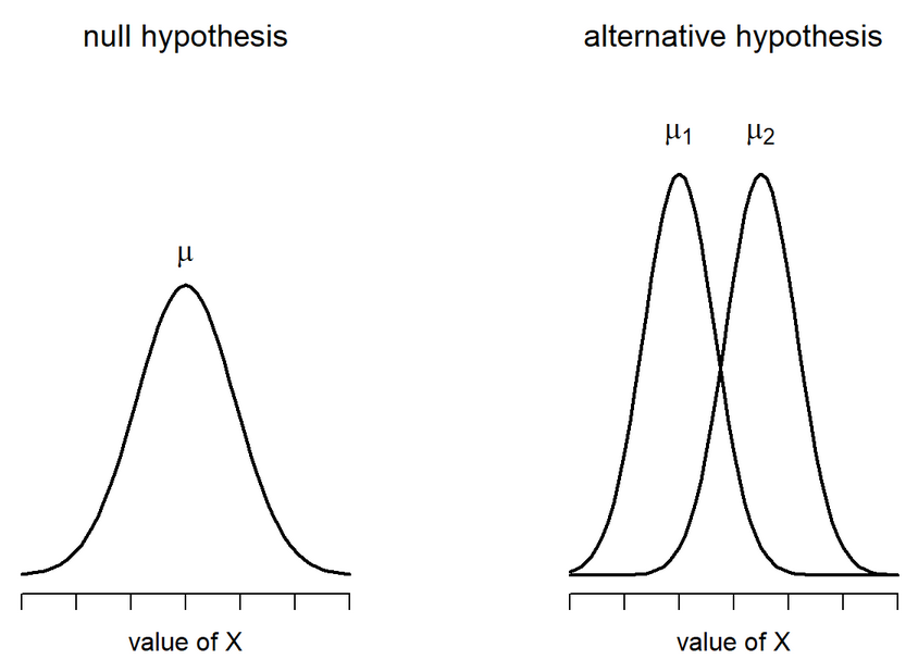
Hypotheses
\(H_0: \mu = 45.05\)
\(H_1: \mu \neq 45.05\)
\[\mu = 45.05\]
\[N = 227\]
\[ \bar{X} = 44.2 \]
\[ s = 15.3 \]
\[ \sigma = Unknown \]
    One Sample t-test

data:  school$Score_in_memory_game
t = -0.86545, df = 223, p-value = 0.3877
alternative hypothesis: true mean is not equal to 45.05
95 percent confidence interval:
 42.14729 46.18116
sample estimates:
mean of x
 44.16422
   One sample t-test

Data variable:   school$Score_in_memory_game

Descriptive statistics:
            Score_in_memory_game
   mean                   44.164
   std dev.               15.318

Hypotheses:
   null:        population mean equals 45.05
   alternative: population mean not equal to 45.05

Test results:
   t-statistic:  -0.865
   degrees of freedom:  223
   p-value:  0.388

Other information:
   two-sided 95% confidence interval:  [42.147, 46.181]
   estimated effect size (Cohen's d):  0.058
Writing Up a t-test
“A one-sample t-test was conducted to determine if the mean [variable name] differed from a hypothesized population mean of [population mean]. The sample mean was M = [sample mean], which was significantly [greater than/less than/different from] the hypothesized population mean, t(df) = [t-value], p = [p-value].”
A one-sample t-test was conducted to determine if the mean score in a memory game for NY students differed from the US population mean. The sample mean was \(M = 44.164\) (SD = 15.32, CI = [42.15, 46.18]), which was not significantly different from the population mean, \(t(223) = -0.87\), \(p = 0.388\).
Single sample t-tests are not used super often in practice
You will mainly see them when interpreting effect sizes of coefficients in your model
#Load sleep data: https://vincentarelbundock.github.io/Rdatasets/datasets.html
sleep <- read_csv("https://raw.githubusercontent.com/dharaden/dharaden.github.io/main/data/sleepstudy.csv")
model = lm(Reaction ~ Days, data = sleep)
summary(model)
Call:
lm(formula = Reaction ~ Days, data = sleep)

Residuals:
     Min       1Q   Median       3Q      Max
-110.848  -27.483    1.546   26.142  139.953

Coefficients:
            Estimate Std. Error t value             Pr(>|t|)
(Intercept)  251.405      6.610  38.033 < 0.0000000000000002 ***
Days          10.467      1.238   8.454  0.00000000000000989 ***
---
Signif. codes:  0 '***' 0.001 '**' 0.01 '*' 0.05 '.' 0.1 ' ' 1

Residual standard error: 47.71 on 178 degrees of freedom
Multiple R-squared:  0.2865,    Adjusted R-squared:  0.2825
F-statistic: 71.46 on 1 and 178 DF,  p-value: 0.000000000000009894
Types of t-Tests
Single Samples t-test
Independent Samples t-test
Paired Samples t-test
Types of t-Tests: Assumptions
Single Samples t-test
Independent Samples t-test
Random Sampling
Independent observations
Approximately normal distributions
Homogeneity of variances
Paired Samples t-test
Approximately normal distributions
Homogeneity of variances
Dataset
Moving forward for today, we will use this dataset
100 students from New York
100 students from New Mexico
Normality Assumption
Check for Normality: Visualizing data (histograms), Q-Q plots, and statistical tests (Shapiro-Wilk, Anderson-Darling) to assess normality.
Remedies for Violations: data transformation or non-parametric alternatives when data is not normally distributed.
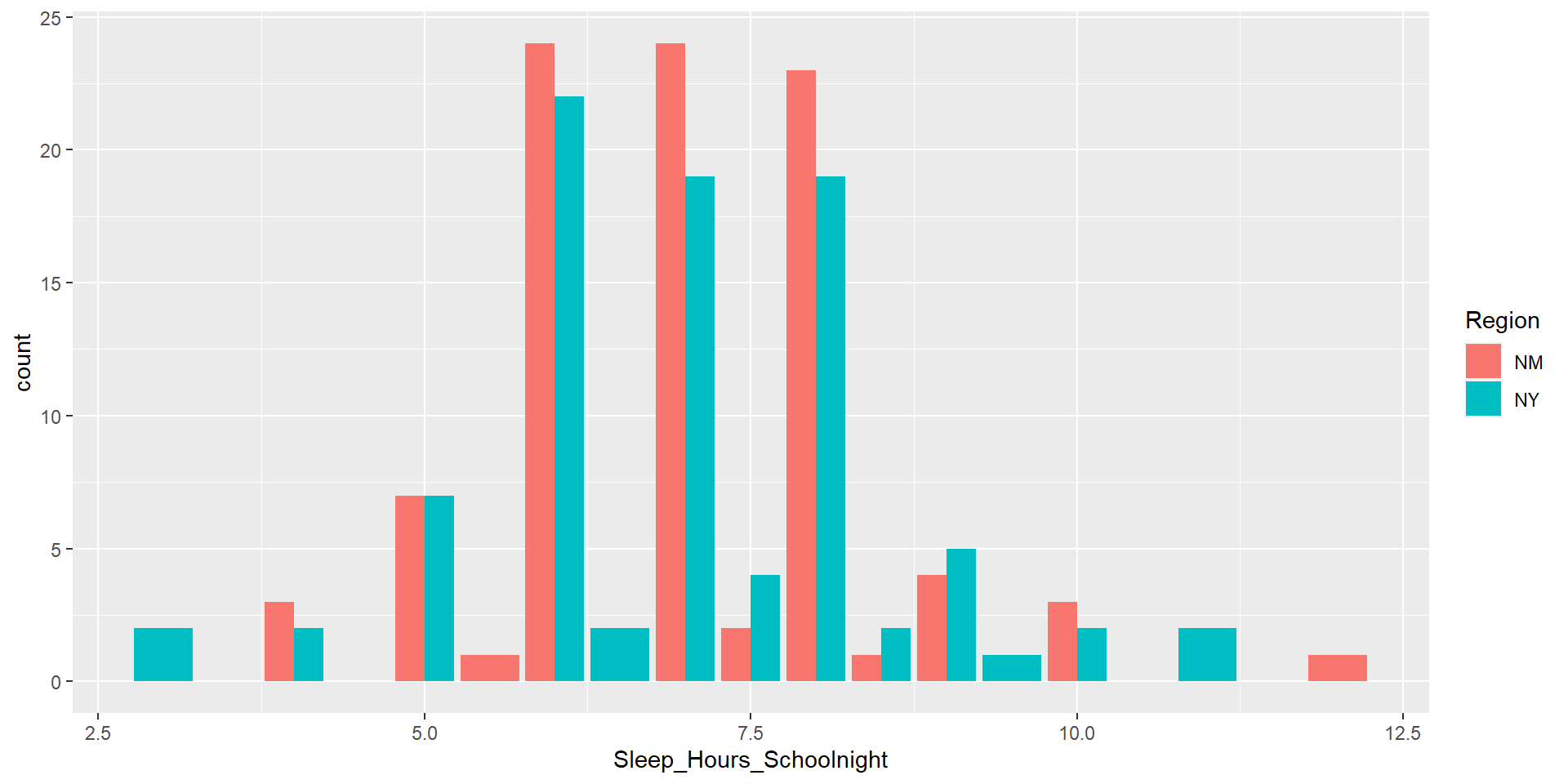
Normality Assumption - Visualizing
Visualizing Data
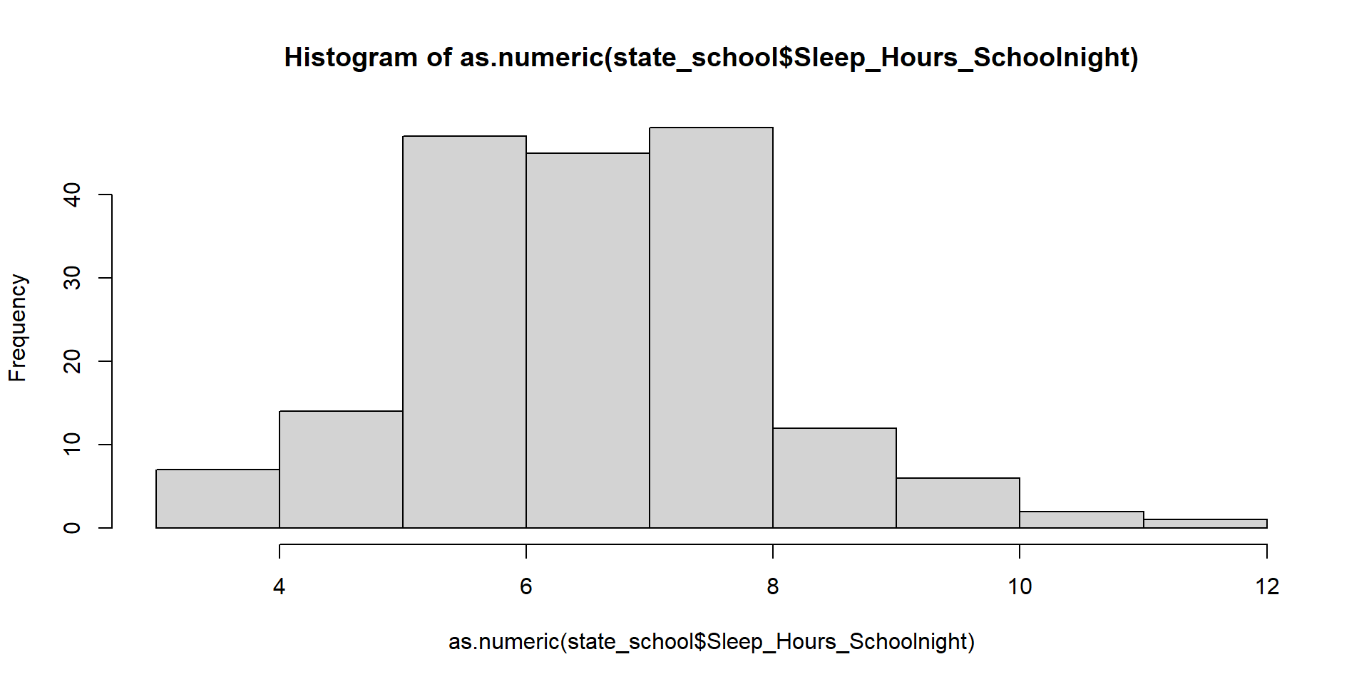
Let’s make it pretty
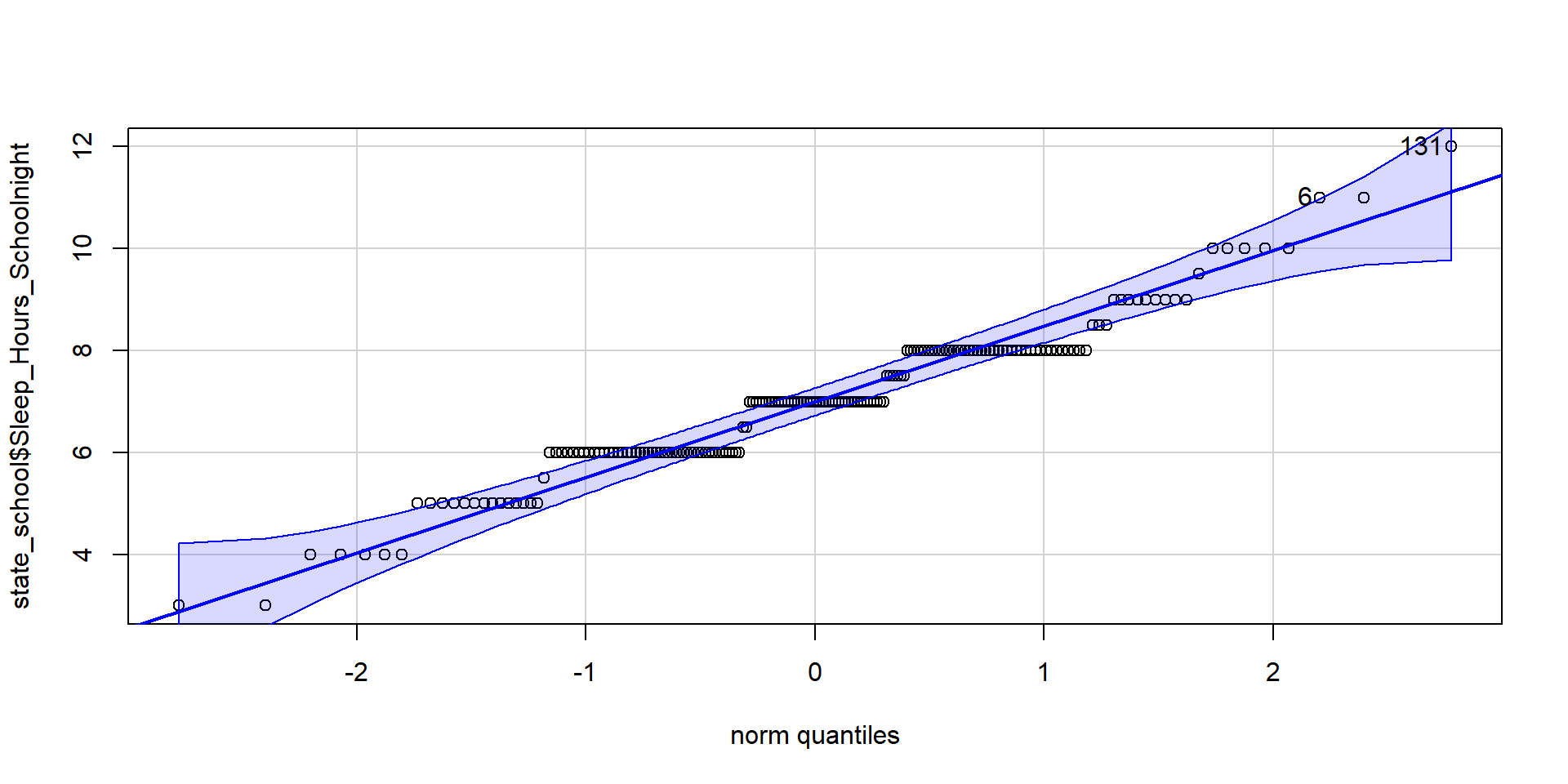
Normality Assumption — Q-Q Plot
A Q-Q plot is a graphical method for assessing whether a dataset follows a normal distribution. It compares the quantiles of your data to the quantiles of a theoretical normal distribution. If your data follows a normal distribution, the points in the Q-Q plot should form a straight line.
Normality Assumption — Shapiro-Wilk Test
Examines the Null Hypothesis that the data are normally distributed
Normality Assumption
Strict adherence to normality assumptions is not always necessary,
- Larger samples bring in Central Limit Theorem
However, assessing normality is still a valuable step in understanding distributions and potential impacts on your analyses
Failure of Normality Assumptions
What can we do if our data violate these normality assumptions?
Logarithmic Transformations
Square Root Transformations
Non-parametric tests
- Mann-Whitney U Test (Wilcoxon Rank-Sum Test): Used for comparing two independent groups
- Wilcoxon Signed-Rank Test: Used for comparing two paired or matched groups
Homogeneity of Variance
Check for Equality of Variances: Levene’s test to assess if variances are equal between groups
Remedies for Violations: Welch’s t-test for unequal variances.
Levene’s Test
This test is used to examine if the variance is equal across groups. The Null Hypothesis is that the variances are equal
# Perform Levene's test for equality of variances
leveneTest(Sleep_Hours_Schoolnight ~ Region,
           data = state_school)
Levene's Test for Homogeneity of Variance (center = median)
Df F value Pr(>F)
group 1 0.5937 0.442
180 Like other tests of significance, Levene’s test gets more powerful as sample size increases. So unless your two variances are exactly equal to each other (and if they are, you don’t need to do a test), your test will be “significant” with a large enough sample. Part of the analysis has to be an eyeball test – is this “significant” because they are truly different, or because I have many subjects.
Independent Samples t-test
Chapter 13.3 in Learning Stats with R
Two different types: Student’s & Welch’s
- Start with Student’s t-test which assumes equal variances between the groups
\[ t = \frac{\bar{X_1} - \bar{X_2}}{SE(\bar{X_1} - \bar{X_2})} \]
Student’s t-test
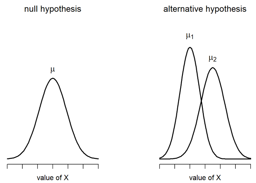
\[ H_0 : \mu_1 = \mu_2 \ \ H_1 : \mu_1 \neq \mu_2 \]
Student’s t-test: Calculate SE
Are able to use a pooled variance estimate
Both variances/standard deviations are assumed to be equal
Therefore:
\[ SE(\bar{X_1} - \bar{X_2}) = \hat{\sigma} \sqrt{\frac{1}{N_1} + \frac{1}{N_2}} \]
We are calculating the Standard Error of the Difference between means
Degrees of Freedom: Total N - 2
Student’s t-test: In R
Using the independentSamplesTest() within the lsr library (make sure it is installed) we can run the test very easily
Formula is outcome ~ group
independentSamplesTTest(
  formula = Sleep_Hours_Schoolnight ~ Region,
  data = state_school,
  var.equal = TRUE #default is FALSE
)
   Student's independent samples t-test

Outcome variable:   Sleep_Hours_Schoolnight
Grouping variable:  Region

Descriptive statistics:
               NM    NY
   mean     6.989 6.994
   std dev. 1.379 1.512

Hypotheses:
   null:        population means equal for both groups
   alternative: different population means in each group

Test results:
   t-statistic:  -0.024
   degrees of freedom:  180
   p-value:  0.981

Other information:
   two-sided 95% confidence interval:  [-0.428, 0.418]
   estimated effect size (Cohen's d):  0.004
Student’s t-test: In R (classic)
Let’s then try it out using the traditional t.test() function. It doesn’t look as nice, but you will likely encounter it when searching for help
    Two Sample t-test

data:  Sleep_Hours_Schoolnight by Region
t = -0.023951, df = 180, p-value = 0.9809
alternative hypothesis: true difference in means between group NM and group NY is not equal to 0
95 percent confidence interval:
 -0.4281648  0.4178954
sample estimates:
mean in group NM mean in group NY
        6.989247         6.994382
Student’s t-test: Write-up
The mean amount of sleep in New Mexico for youth was 6.989 (SD = 1.379), while the mean in New York was 6.994 (SD = 1.512). A Student’s independent samples t-test showed that there was not a significant mean difference (t(180)=-0.024, p=.981, \(CI_{95}\)=[-0.43, 0.42], d=.004). This suggests that there is no difference between youth in NM and NY on amount of sleep on school nights.
Welch’s t-test
\[ H_0 : \mu_1 = \mu_2 \ \ H_1 : \mu_1 \neq \mu_2 \]
Welch’s t-test: Calculate SE
Since the variances are not equal, we have to estimate the SE differently
\[ SE(\bar{X_1} - \bar{X_2}) = \sqrt{\frac{\hat{\sigma_1^2}}{N_1} + \frac{\hat{\sigma_2^2}}{N_2}} \]
Degrees of Freedom is also very different:
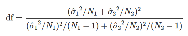
Welch’s t-test: In R
We use the same function as before, but specify that the variances are not equal
independentSamplesTTest(
  formula = Sleep_Hours_Schoolnight ~ Region,
  data = state_school,
  var.equal = FALSE
)
   Welch's independent samples t-test

Outcome variable:   Sleep_Hours_Schoolnight
Grouping variable:  Region

Descriptive statistics:
               NM    NY
   mean     6.989 6.994
   std dev. 1.379 1.512

Hypotheses:
   null:        population means equal for both groups
   alternative: different population means in each group

Test results:
   t-statistic:  -0.024
   degrees of freedom:  176.737
   p-value:  0.981

Other information:
   two-sided 95% confidence interval:  [-0.429, 0.419]
   estimated effect size (Cohen's d):  0.004
Welch’s t-test: In R (classic)
Let’s then try it out using the traditional t.test() function…turns out it is pretty straightforward
Welch Two Sample t-test
data: Sleep_Hours_Schoolnight by Region
t = -0.023902, df = 176.74, p-value = 0.981
alternative hypothesis: true difference in means between group NM and group NY is not equal to 0
95 percent confidence interval:
-0.4290776 0.4188082
sample estimates:
mean in group NM mean in group NY
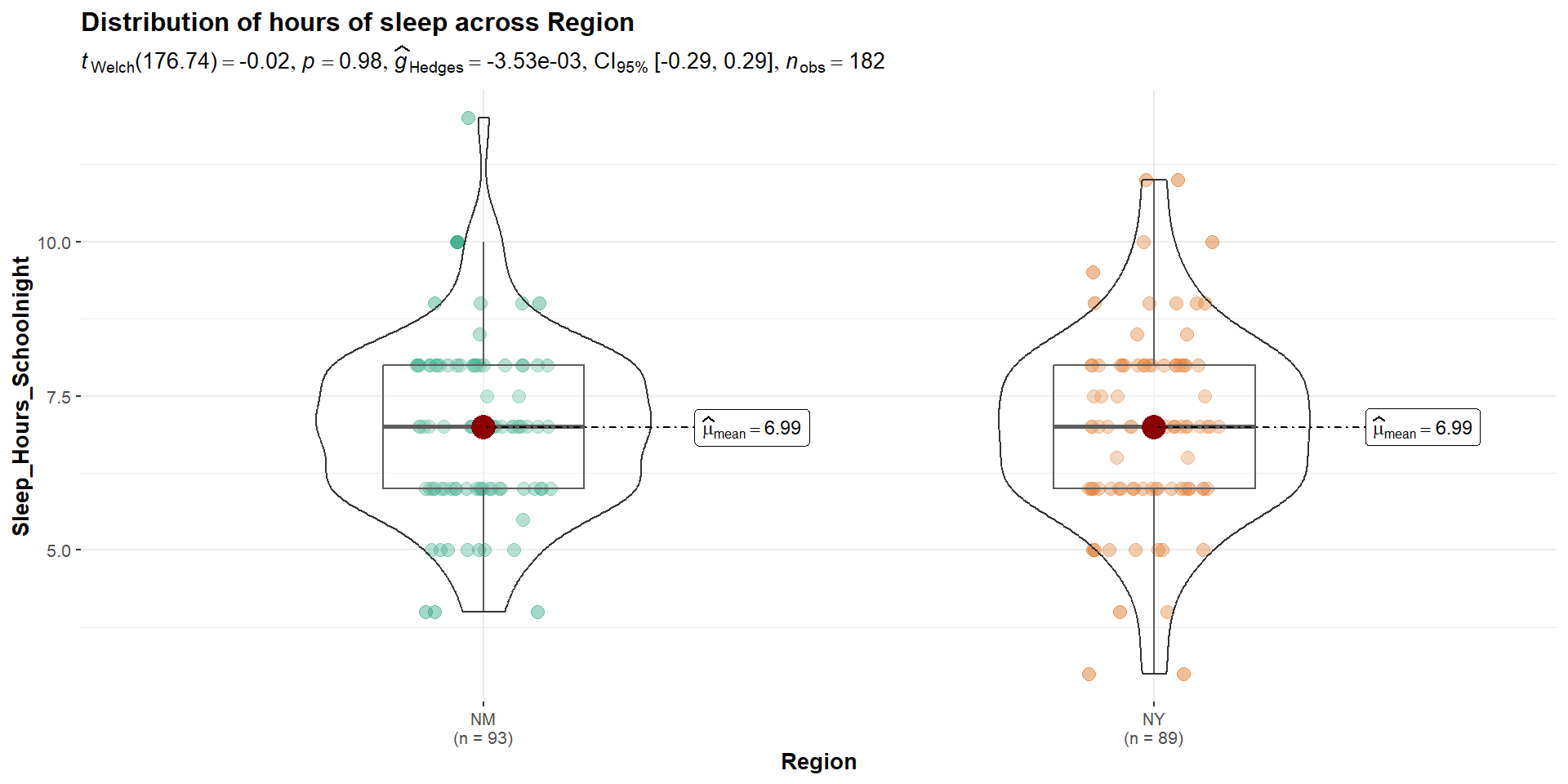
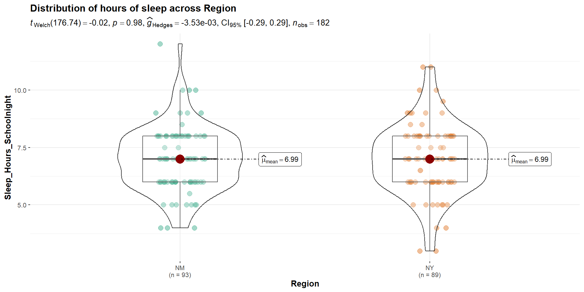
6.989247 6.994382 Cool Visualizations
The library ggstatsplot has some wonderful visualizations of various tests
In-Class Lab
Take a look at the data in state_school and identify another Independent Samples t-test that you can perform
- Be sure to select (1) a grouping variable and (2) a continuous variable to look at differences between the groups
Follow the steps that we went through today:
- Check for Normality of the variable
- Check for Homogeneity of Variances
- Perform the appropriate t-test
- Report Results
Knit the document
Next Time…
Paired Samples t-test
Paired Samples t-Test in R
Chapter 13.5 - Learning Stats with R
Also called “Dependent Samples t-test”
We have been testing means between two independent samples. Participants may be randomly assigned to the separate groups
- This is limited to those types of study designs, but what if we have repeated measures?
We will then need to compare scores across people…the samples we are comparing now depend on one another and are paired
Common Mistakes and Pitfalls
Misinterpreting p-Values
Violations of Assumptions
Sample Size Considerations
Multiple Testing Issues