Comparing Means: Paired t-tests
PSYC 640 - Fall 2023
Last week
- Comparing Means: \(t\)-test
- Independent Samples \(t\)-test
Today…
Comparing Means with the \(t\)-test
- Paired Samples
Review: Independent \(t\)-test
Independent Samples \(t\)-test
Chapter 13.3 in Learning Stats with R
Two different types: Student’s & Welch’s
- Student’s \(t\)-test
- Welch’s \(t\)-test
\[ t = \frac{\bar{X_1} - \bar{X_2}}{SE(\bar{X_1} - \bar{X_2})} \]
Types of t-Tests: Assumptions
Single Samples t-test
Independent Samples t-test
Paired Samples t-test
Approximately normal distributions
Homogeneity of variances
Spoiler Alert! The same as a one-sample \(t\)-test
Steps for \(t\)-test
- Check for normality of variables
- Visualizing, Q-Q plots, Statistical Tests
- Homogeneity of Variance
- Levene’s test –> Welch’s \(t\)-test
Student’s t-test: In R
independentSamplesTest()
independentSamplesTTest(
  formula = Sleep_Hours_Schoolnight ~ Region,
  data = state_school,
  var.equal = TRUE #default is FALSE
)
   Student's independent samples t-test

Outcome variable:   Sleep_Hours_Schoolnight
Grouping variable:  Region

Descriptive statistics:
               NM    NY
   mean     6.989 6.994
   std dev. 1.379 1.512

Hypotheses:
   null:        population means equal for both groups
   alternative: different population means in each group

Test results:
   t-statistic:  -0.024
   degrees of freedom:  180
   p-value:  0.981

Other information:
   two-sided 95% confidence interval:  [-0.428, 0.418]
   estimated effect size (Cohen's d):  0.004
t.test()
    Two Sample t-test

data:  Sleep_Hours_Schoolnight by Region
t = -0.023951, df = 180, p-value = 0.9809
alternative hypothesis: true difference in means between group NM and group NY is not equal to 0
95 percent confidence interval:
 -0.4281648  0.4178954
sample estimates:
mean in group NM mean in group NY
        6.989247         6.994382
Welch’s t-test: In R
independentSamplesTest()
independentSamplesTTest(
  formula = Sleep_Hours_Schoolnight ~ Region,
  data = state_school,
  var.equal = FALSE #This is what is different!
)
   Welch's independent samples t-test

Outcome variable:   Sleep_Hours_Schoolnight
Grouping variable:  Region

Descriptive statistics:
               NM    NY
   mean     6.989 6.994
   std dev. 1.379 1.512

Hypotheses:
   null:        population means equal for both groups
   alternative: different population means in each group

Test results:
   t-statistic:  -0.024
   degrees of freedom:  176.737
   p-value:  0.981

Other information:
   two-sided 95% confidence interval:  [-0.429, 0.419]
   estimated effect size (Cohen's d):  0.004
t.test()
t.test(
  formula = Sleep_Hours_Schoolnight ~ Region,
  data = state_school,
  var.equal = FALSE #This is what is different!
)
    Welch Two Sample t-test

data:  Sleep_Hours_Schoolnight by Region
t = -0.023902, df = 176.74, p-value = 0.981
alternative hypothesis: true difference in means between group NM and group NY is not equal to 0
95 percent confidence interval:
 -0.4290776  0.4188082
sample estimates:
mean in group NM mean in group NY
        6.989247         6.994382
Interpreting and writing up an independent samples t-test
The first sentence usually conveys some descriptive information about the two groups you were comparing. Then you identify the type of test you conducted and what was determined (be sure to include the “stat block” here as well with the t-statistic, df, p-value, CI and Effect size). Finish it up by putting that into person words and saying what that means.
The mean amount of sleep in New Mexico for youth was 6.989 (SD = 1.379), while the mean in New York was 6.994 (SD = 1.512). A Student’s independent samples t-test showed that there was not a significant mean difference (t(180)=-0.024, p=.981, \(CI_{95}\)=[-0.43, 0.42], d=.004). This suggests that there is no difference between youth in NM and NY on amount of sleep on school nights.
Today: Paired Samples
Paired Samples \(t\)-Test
Chapter 13.5 - Learning Stats with R
Also called “Dependent Samples t-test”
We have been testing means between two independent samples. Participants may be randomly assigned to the separate groups
- This is limited to those types of study designs, but what if we have repeated measures?
We will then need to compare scores across people…the samples we are comparing now depend on one another and are paired
Paired Samples \(t\)-test
Each of the repeated measures (or pairs) can be viewed as a difference score
This reduces the analysis to a one-sample t-test of the difference score
- We are comparing the sample (i.e., difference scores) to a population \(\mu\) = 0
Assumptions: Paired Samples
The variable of interest (difference scores):
Continuous (Interval/Ratio)
Have 2 groups (and only two groups) that are matched
Normally Distributed
Why paired samples??
Previously, we looked at independent samples \(t\)-tests, which we could do here as well (nobody will yell at you)
However, this would violate the assumption that the data points are independent of one another!
Within vs. Between-subjects
Within vs. Between Subjects
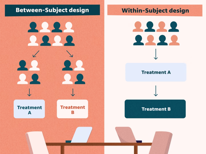
Paired Samples: Single Sample
Instead of focusing on these variables as being separate/independent, we need to be able to account for their dependency on one another
This is done by calculating a difference or change score for each participant
\[ D_i = X_{i1} - X_{i2} \]
Notice: The equation is set up as variable1 minus variable2. This will be important when we interpret the results
Paired Samples: Hypotheses & \(t\)-statistic
The hypotheses would then be:
\[ H_0: \mu_D = 0; H_1: \mu_D \neq 0 \]
And to calculate our t-statistic: \(t_{df=n-1} = \frac{\bar{D}}{SE(D)}\)
where the Standard Error of the difference score is: \(\frac{\hat{\sigma_D}}{\sqrt{N}}\)
Review of the t-test process
Collect Sample and define hypotheses
Set alpha level
Determine the sampling distribution (\(t\) distribution for now)
Identify the critical value that corresponds to alpha and df
Calculate test statistic for sample collected
Inspect & compare statistic to critical value; Calculate probability
Example 1: Simple
Participants are placed in two differently colored rooms and are asked to rate overall happiness levels after each
Hypotheses:
\(H_0:\) There is no difference in ratings of happiness between the rooms ( \(\mu = 0\) )
\(H_1:\) There is a difference in ratings of happiness between the rooms ( \(\mu \neq 0\) )
| Participant | Blue Room Score | Orange Room Score | Difference (\(X_{iB} - X_{iO}\)) |
|---|---|---|---|
| 1 | 3 | 6 | -3 |
| 2 | 9 | 9 | 0 |
| 3 | 2 | 10 | -8 |
| 4 | 9 | 6 | 3 |
| 5 | 5 | 2 | 3 |
| 6 | 5 | 7 | -2 |
Determining \(t\)-crit
Can look things up using a t-table where you need the degrees of freedom and the alpha
But we have R to do those things for us:
Calculating t
Let’s get all of the information for the sample we are focusing on (difference scores):
Calculating t
Now we can calculate our \(t\)-statistic: \[t_{df=n-1} = \frac{\bar{D}}{\frac{sd_{diff}}{\sqrt{n}}}\]
Make a decision
Hypotheses:
\(H_0:\) There is no difference in ratings of happiness between the rooms ( \(\mu = 0\) )
\(H_1:\) There is a difference in ratings of happiness between the rooms ( \(\mu \neq 0\) )
| \(alpha\) | \(t-crit\) | \(t-statistic\) | \(p-value\) |
|---|---|---|---|
| 0.05 | \(\pm\) -2.57 | -0.69 | 0.52 |
What can we conclude??
Example 2: Data in R
We will use the same dataset that we have in the last few classes
Let’s Look at the data
Research Question: Is there a difference between school nights and weekend nights for amount of time slept?
Only looking at the variables that we are potentially interested in:
state_school %>%
  select(Gender, Ageyears, Sleep_Hours_Schoolnight, Sleep_Hours_Non_Schoolnight) %>%
  head() #look at first few observations
Gender Ageyears Sleep_Hours_Schoolnight Sleep_Hours_Non_Schoolnight
1 Female 16 8.0 13
2 Male 17 8.0 9
3 Female 19 8.0 7
4 Male 17 8.0 9
5 Male 16 8.5 5
6 Female 11 11.0 12Difference Score
This can be done in a couple different ways and sometimes you will see things computed this way:
However, we like the tidyverse so why don’t we use the mutate() function
And I always overdo things, so I am going to make a new dataset that only has the variables that I’m interested in (sleep_state_school)
Code
  Gender Ageyears Sleep_Hours_Schoolnight Sleep_Hours_Non_Schoolnight
1 Female       16                     8.0                          13
2   Male       17                     8.0                           9
3 Female       19                     8.0                           7
4   Male       17                     8.0                           9
5   Male       16                     8.5                           5
6 Female       11                    11.0                          12
sleep_diff
1 -5.0
2 -1.0
3 1.0
4 -1.0
5 3.5
6 -1.0Visualizing
Now that we have our variable of interest, let’s take a look at it!
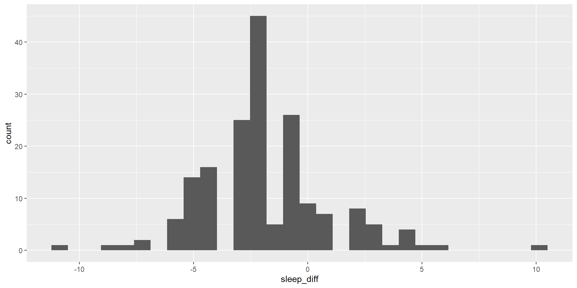
Doing the test in R: One Sample
Since we have calculated the difference scores, we can basically just do a one-sample t-test with the lsr library
   One sample t-test

Data variable:   sleep_state_school$sleep_diff

Descriptive statistics:
            sleep_diff
   mean         -1.866
   std dev.      2.741

Hypotheses:
   null:        population mean equals 0
   alternative: population mean not equal to 0

Test results:
   t-statistic:  -9.106
   degrees of freedom:  178
   p-value:  <.001

Other information:
   two-sided 95% confidence interval:  [-2.27, -1.462]
   estimated effect size (Cohen's d):  0.681
Doing the test in R: Paired Sample
Maybe we want to keep things separate and don’t want to calculate separate values. We can use pairedSamplesTTest() instead!
pairedSamplesTTest(
  formula = ~ Sleep_Hours_Schoolnight + Sleep_Hours_Non_Schoolnight,
  data = sleep_state_school
)
   Paired samples t-test

Variables:  Sleep_Hours_Schoolnight , Sleep_Hours_Non_Schoolnight

Descriptive statistics:
            Sleep_Hours_Schoolnight Sleep_Hours_Non_Schoolnight difference
   mean                       6.992                       8.858     -1.866
   std dev.                   1.454                       2.412      2.741

Hypotheses:
   null:        population means equal for both measurements
   alternative: different population means for each measurement

Test results:
   t-statistic:  -9.106
   degrees of freedom:  178
   p-value:  <.001

Other information:
   two-sided 95% confidence interval:  [-2.27, -1.462]
   estimated effect size (Cohen's d):  0.681
Doing the test in R: Classic Edition
As you Google around to figure things out, you will likely see folks using `t.test()
t.test(
  x = sleep_state_school$Sleep_Hours_Schoolnight,
  y = sleep_state_school$Sleep_Hours_Non_Schoolnight,
  paired = TRUE
)
    Paired t-test

data:  sleep_state_school$Sleep_Hours_Schoolnight and sleep_state_school$Sleep_Hours_Non_Schoolnight
t = -9.1062, df = 178, p-value < 0.00000000000000022
alternative hypothesis: true mean difference is not equal to 0
95 percent confidence interval:
 -2.270281 -1.461563
sample estimates:
mean difference
      -1.865922
Reporting \(t\)-test
The first sentence usually conveys some descriptive information about the sample you were comparing (e.g., pre & post test).
Then you identify the type of test you conducted and what was determined (be sure to include the “stat block” here as well with the t-statistic, df, p-value, CI and Effect size).
Finish it up by putting that into person words and saying what that means.
Common Mistakes and Pitfalls
Misinterpreting p-Values
Violations of Assumptions
Sample Size Considerations
Multiple Testing Issues
If we have time: Example 3 - Dog Training
A dog trainer wants to know if dogs are faster at an agility course if a jump is early in the course or later. She has a sample of dogs from her classes run both courses and measures their finish times. Half the class runs the early barrier version on Tuesday, half the class runs the early barrier version on Thursday. Is there a significant difference between course types (alpha = 0.05)?
Next time…
Visualizing with ggplot
Parameterization of reports (not using “magic numbers”)