Introduction to ANOVA

PSYC 640 - Fall 2023

Dustin Haraden, PhD

Last Week

• Comparing Means with 2 groups: \(t\)-test
  • Independent Samples \(t\)-test Review
  • Paired Samples \(t\)-test

Looking Ahead

• Plan to have 2 more labs that will be similar to the last lab

  • Likely take place on 10/25 and sometime the week of 11/13

• Outside of these labs, I am going to plan on having additional mini-labs

  • Likely to take place on 11/1, 11/22 and 11/29 (will update based on how things are going in class)

Today…

Introduction to ANOVA (Analysis of Variance)

# File management
library(here)
# for dplyr, ggplot2
library(tidyverse)
#Loading data
library(rio)

#Remove Scientific Notation 
options(scipen=999)

Overview of ANOVA

What is ANOVA? (LSR Ch. 14)

• ANOVA stands for Analysis of Variance
• Comparing means between two or more groups (usually 3 or more)
  • Continuous outcome and grouping variable with 2 or more levels
• Under the larger umbrella of general linear models
  • ANOVA is basically a regression with only categorical predictors
• Likely the most widely used tool in Psychology

Different Types of ANOVA

• One-Way ANOVA

• Two-Way ANOVA

• Repeated Measures ANOVA

• ANCOVA

• MANOVA

One-Way ANOVA

Goal: Inform of differences among the levels of our variable of interest (Omnibus Test)

• But cannot tell us more than that…

Hypotheses:

\[ H_0: it\: is\: true\: that\: \mu_1 = \mu_2 = \mu_3 =\: ...\mu_k \\ H_1: it\: is\: \boldsymbol{not}\: true\: that\: \mu_1 = \mu_2 = \mu_3 =\: ...\mu_k \]

Wait…Means or Variance?

We are using the variance to create a ratio (within group versus between group variance) to determine differences in means

• We are not directly investigating variance, but operationalize variance to create the ratio:

\[ F_{df_b, \: df_w} = \frac{MS_{between}}{MS_{within}} \]

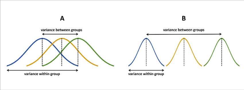
\(F = \frac{MS_{between}}{MS_{within}} = \frac{small}{large} < 1\)

\(F = \frac{MS_{between}}{MS_{within}} = \frac{large}{small} > 1\)

ANOVA: Assumptions

Independence

• Observations between and within groups should be independent. No autocorrelation

Homogeneity of Variance

• The variances within each group should be roughly equal
  • Levene’s test –> Welch’s ANOVA for unequal variances

Normality

• The data within each group should follow a normal distribution
  • Shapiro-Wilk test –> can transform the data or use non-parametric tests

NHST with ANOVA

Review of the NHST process

1. Collect Sample and define hypotheses

2. Set alpha level

3. Determine the sampling distribution (will be using \(F\)-distribution now)

4. Identify the critical value

5. Calculate test statistic for sample collected

6. Inspect & compare statistic to critical value; Calculate probability

Steps to calculating F-ratio

1. Capture variance both between and within groups
2. Variance to Sum of Squares
3. Degrees of Freedom
4. Mean squares values
5. F-Statistic

Capturing Variance

We have calculated variance before!

\[ Var = \frac{1}{N}\sum(x_i - \bar{x})^2 \]

Now we have to take into account the variance between and within the groups:

\[ Var(Y) = \frac{1}{N} \sum^G_{k=1}\sum^{N_k}_{i=i}(Y_{ik} - \bar{Y})^2 \]

Notice that we have the summation across each group ( \(G\) ) and the person in the group ( \(N_k\) )

Variance to Sum of Squares

Total Sum of Squares - Adding up the sum of squares instead of getting the average (notice the removal of \(\frac{1}{N}\))

\[ SS_{total} = \sum^G_{k=1}\sum^{N_k}_{i=i}(Y_{ik} - \bar{Y})^2 \]

Can be broken up to see what is the variation between the groups AND the variation within the groups

\[ SS_{total}=SS_{between}+SS_{within} \]

This gets us closer to understanding the difference between means

Sum of Squares

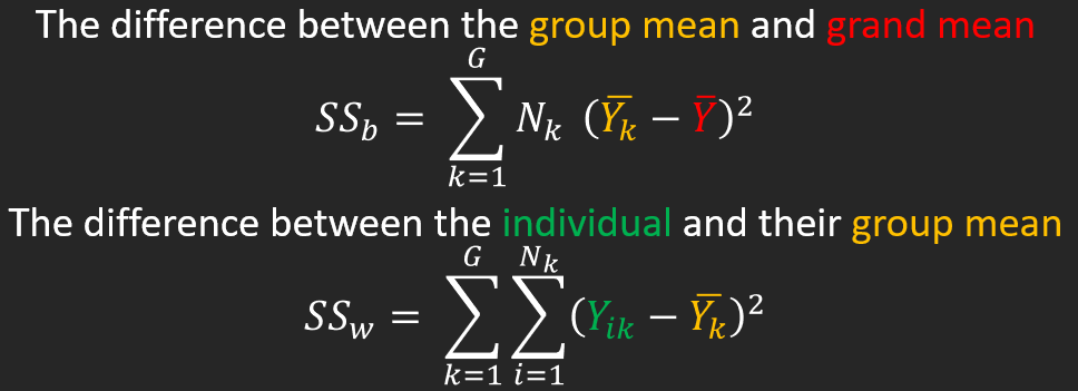
Sum of Squares

\[ SS_{total}=SS_{between}+SS_{within} \]

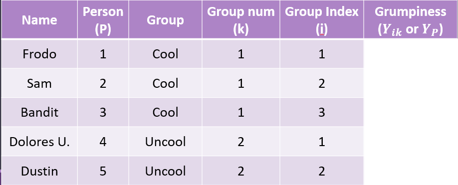
Example Data

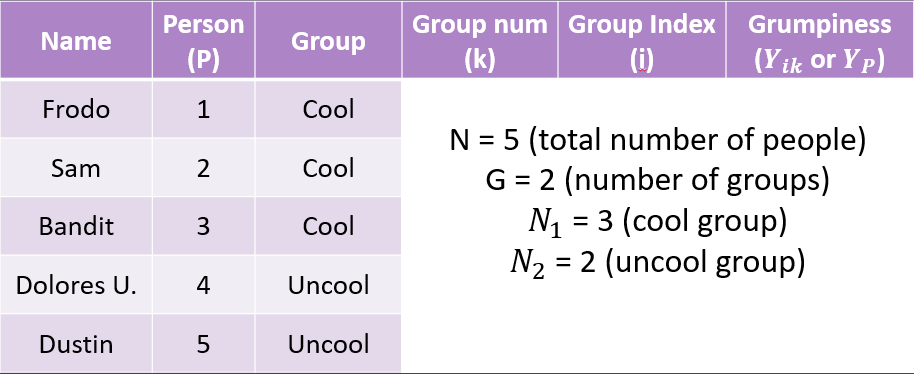
Example Data

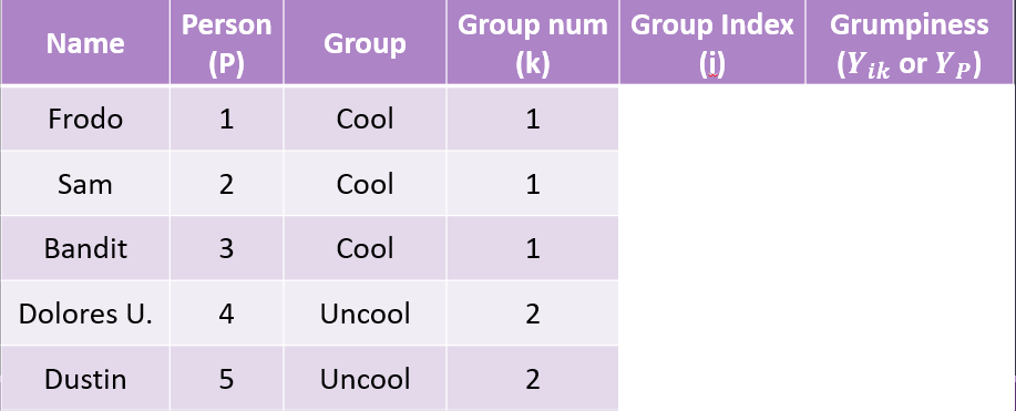
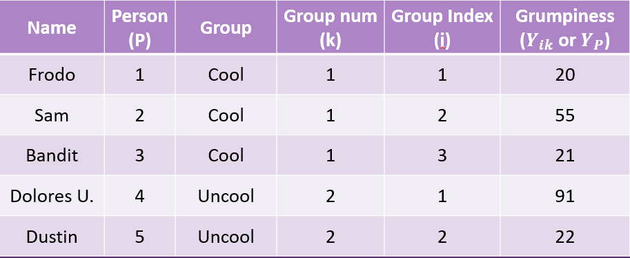
Example Data

Example Data

Sum of Squares - Between

The difference between the group mean and grand mean

\[ SS_{between} = \sum^G_{k=1}N_k(\bar{Y_k} - \bar{Y})^2 \]

Group	Group Mean \(\bar{Y_k}\)	Grand Mean \(\bar{Y}\)
Cool	32	41.8
Uncool	56.5	41.8

Sum of Squares - Between

The difference between the group mean and grand mean

\[ SS_{between} = \sum^G_{k=1}N_k(\bar{Y_k} - \bar{Y})^2 \]

Group	Group Mean \(\bar{Y_k}\)	Grand Mean \(\bar{Y}\)	Sq. Dev.	N	Weighted Sq. Dev.
Cool	32	41.8	96.04	3	288.12
Uncool	56.5	41.8	216.09	2	432.18

Sum of Squares - Between

The difference between the group mean and grand mean

\[ SS_{between} = \sum^G_{k=1}N_k(\bar{Y_k} - \bar{Y})^2 \]

Now we can sum the Weighted Squared Deviations together to get our Sum of Squares Between:

ssb <- 288.12 + 432.18
ssb

[1] 720.3

Sum of Squares - Within

The difference between the individual and their group mean

\[ SS_{within} = \sum^G_{k=1}\sum^{N_k}_{i=i}(Y_{ik} - \bar{Y_k})^2 \]

Name	Grumpiness \(Y_{ik}\)	Group Mean \(\bar{Y_K}\)
Frodo	20	32
Sam	55	32
Bandit	21	32
Dolores U.	91	56.5
Dustin	22	56.5

Sum of Squares - Within

The difference between the individual and their group mean

\[ SS_{within} = \sum^G_{k=1}\sum^{N_k}_{i=i}(Y_{ik} - \bar{Y_k})^2 \]

Name	Grumpiness \(Y_{ik}\)	Group Mean \(\bar{Y_K}\)	Sq. Dev
Frodo	20	32	144
Sam	55	32	529
Bandit	21	32	121
Dolores U.	91	56.5	1190.25
Dustin	22	56.5	1190.25

Code

score <- c(20, 55, 21, 91, 22)
group_m <- c(32, 32, 32, 56.5, 56.5)
sq_dev <- (score - group_m)^2

Sum of Squares - Within

The difference between the individual and their group mean

\[ SS_{within} = \sum^G_{k=1}\sum^{N_k}_{i=i}(Y_{ik} - \bar{Y_k})^2 \] Now we can sum the Squared Deviations together to get our Sum of Squares Within:

sum(sq_dev)

[1] 3174.5

Sum of Squares

Can start to have an idea of what this looks like

\[ SS_{between} = \sum^G_{k=1}N_k(\bar{Y_k} - \bar{Y})^2 = 720.3 \]

\[ SS_{within} = \sum^G_{k=1}\sum^{N_k}_{i=i}(Y_{ik} - \bar{Y_k})^2 = 3174.5 \]

Next we have to take into account the degrees of freedom

Degrees of Freedom - ANOVA

Degrees of Freedom

Since we have 2 types of variations that we are examining, this needs to be reflected in the degrees of freedom

1. Take the number of groups and subtract 1
   \(df_{between} = G - 1\)

2. Take the total number of observations and subtract the number of groups
   

   \(df_{within} = N - G\)

Mean Squares

Calculating Mean Squares

Next we convert our summed squares value into a “mean squares”

This is done by dividing by the respective degrees of freedom

\[ MS_b = \frac{SS_b}{df_b} \]

\[ MS_W = \frac{SS_w}{df_w} \]

Calculating Mean Squares - Example

Let’s take a look at how this applies to our example: \[ MS_b = \frac{SS_b}{G-1} = \frac{720.3}{2-1} = 720.3 \]

\[ MS_W = \frac{SS_w}{N-G} = \frac{3174.5}{5-2} = 1058.167 \]

\(F\)-Statistic

Calculating the F-Statistic

\[F = \frac{MS_b}{MS_w}\]

If the null hypothesis is true, \(F\) has an expected value close to 1 (numerator and denominator are estimates of the same variability)

If it is false, the numerator will likely be larger, because systematic, between-group differences contribute to the variance of the means, but not to variance within group.

Code

data.frame(F = c(0,8)) %>%
  ggplot(aes(x = F)) +
  stat_function(fun = function(x) df(x, df1 = 3, df2 = 196), 
                geom = "line") +
  stat_function(fun = function(x) df(x, df1 = 3, df2 = 196), 
                geom = "area", xlim = c(2.65, 8), fill = "purple") +
  geom_vline(aes(xintercept = 2.65), color = "purple") +
  scale_y_continuous("Density") + scale_x_continuous("F statistic", breaks = NULL) +
  theme_bw(base_size = 20)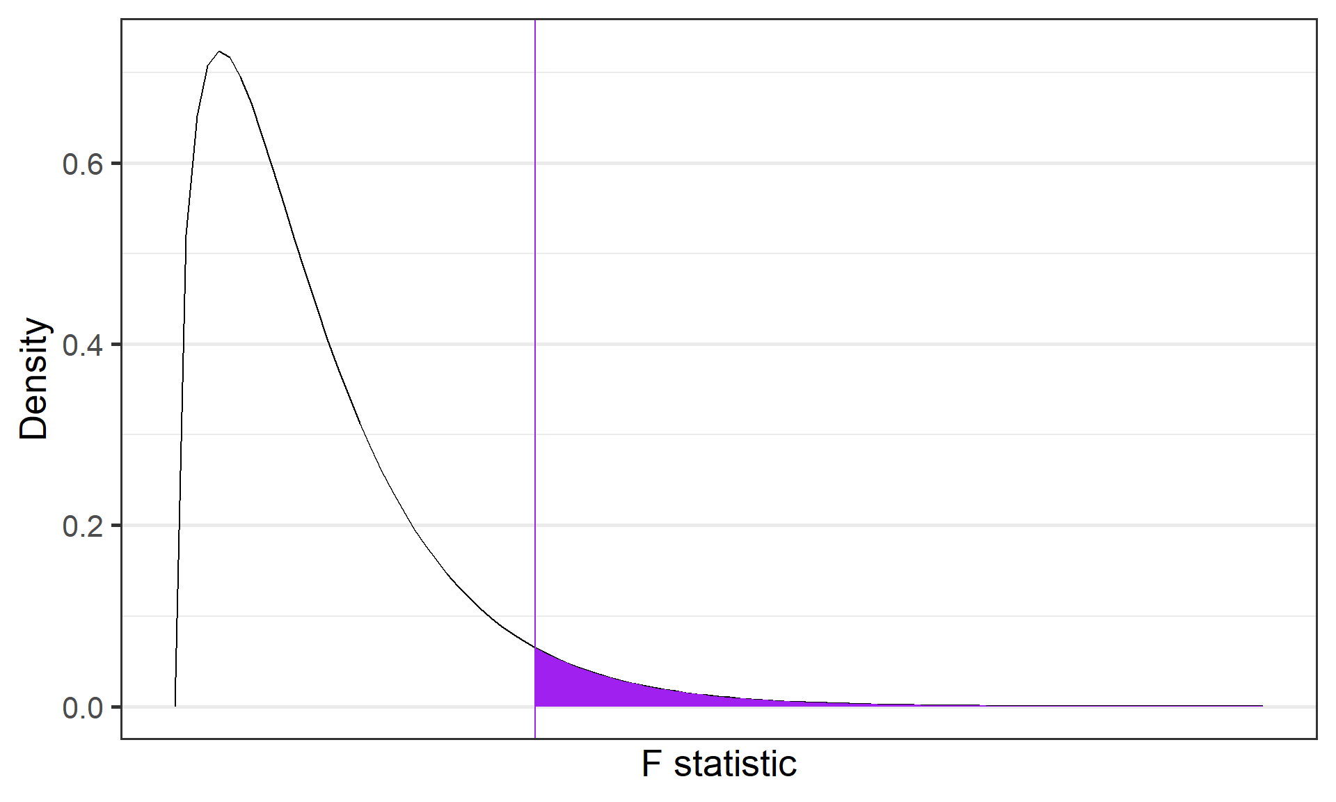

If data are normally distributed, then the variance is \(\chi^2\) distributed

\(F\)-distributions are one-tailed tests. Recall that we’re interested in how far away our test statistic from the null \((F = 1).\)

Calculating F-statistic: Example

\[F = \frac{MS_b}{MS_w} = \frac{720.3}{1058.167} = 0.68\]

Link to probability calculator

Code

data.frame(F = c(0,8)) %>%
  ggplot(aes(x = F)) +
  stat_function(fun = function(x) df(x, df1 = 3, df2 = 196), 
                geom = "line") +
  stat_function(fun = function(x) df(x, df1 = 3, df2 = 196), 
                geom = "area", xlim = c(2.65, 8), fill = "purple") +
  geom_vline(aes(xintercept = 2.65), color = "purple") + 
  geom_vline(aes(xintercept = 0.68), color = "red") + 
  annotate("text",
           label = "F=0.68", 
           x = 1.1, y = 0.65, size = 8, color = "red") + 
  scale_y_continuous("Density") + scale_x_continuous("F statistic", breaks = NULL) +
  theme_bw(base_size = 20)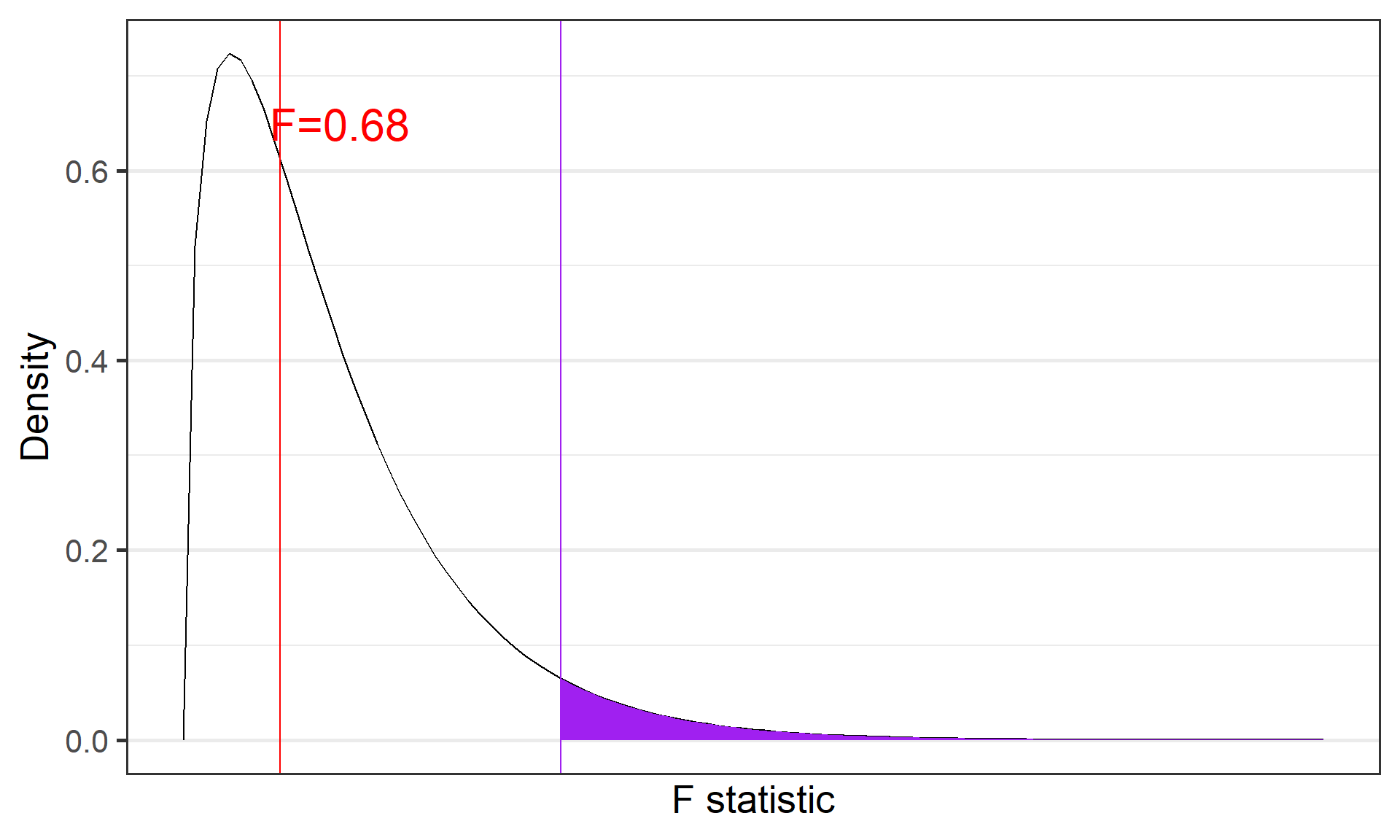

What can we conclude?

Contrasts/Post-Hoc Tests

Performed when there is a significant difference among the groups to examine which groups are different

1. Contrasts: When we have a priori hypotheses
2. Post-hoc Tests: When we want to test everything

Reporting Results

Tables

Often times the output will be in the form of a table and then it is often reported this way in the manuscript

Source of Variation	df	Sum of Squares	Mean Squares	F-statistic	p-value
Group	\(G-1\)	\(SS_b\)	\(MS_b = \frac{SS_b}{df_b}\)	\(F = \frac{MS_b}{MS_w}\)	\(p\)
Residual	\(N-G\)	\(SS_w\)	\(MS_w = \frac{SS_w}{df_w}\)
Total	\(N-1\)	\(SS_{total}\)

In-Text

A one-way analysis of variance was used to test for differences in the [variable of interest/outcome variable] as a function of [whatever the factor is]. Specifically, differences in [variable of interest] were assessed for the [list different levels and be sure to include (M= , SD= )] . The one-way ANOVA revealed a significant/nonsignificant effect of [factor] on scores on the [variable of interest] (F(dfb, dfw) = f-ratio, p = p-value, η2 = effect size).

Planned comparisons were conducted to compare expected differences among the [however many groups] means. Planned contrasts revealed that participants in the [one of the conditions] had a greater/fewer [variable of interest] and then include the p-value. This same type of sentence is repeated for whichever contrasts you completed. Descriptive statistics were reported in Table 1.

Spooky Data Example

New Data Collection: Example

We want to be able to connect with the paranormal. Collected data at different locations to examine whether there are certain areas that have more ghost activity. We have multiple ratings (EMF) at the various locations to determine the potential presence of ghosts. The locations were determined by a select group of undergraduate researchers. They include:

• Walmart
• Abandoned Walmart
• Ikea
• Getysburg

• The Woods
• Unused Stairwell
• RIT Tunnels
• This classroom

Review of the NHST process

1. Collect Sample and define hypotheses

2. Set alpha level

3. Determine the sampling distribution (will be using \(F\)-distribution now)

4. Identify the critical value

5. Calculate test statistic for sample collected

6. Inspect & compare statistic to critical value; Calculate probability

Example:

Take a look at the data and compute the following:

Source of Variation	df	Sum of Squares	Mean Squares	F-statistic	p-value
Group	\(G-1\)	\(SS_b\)	\(MS_b = \frac{SS_b}{df_b}\)	\(F = \frac{MS_b}{MS_w}\)	\(p\)
Residual	\(N-G\)	\(SS_w\)	\(MS_w = \frac{SS_w}{df_w}\)
Total	\(N-1\)	\(SS_{total}\)

Can use R or Excel

Next time…

• Two-Way ANOVA!