Multiple Regression: A story of betas

PSYC 640 - Fall 2023

Dustin Haraden, PhD

Last Time

Coefficient of Determination
Coefficient of Alienation

Today…

More Regression (but more details)
- Omnibus test
Multiple Regression? Comparing Models?
Probably some Group work

options(scipen=999)
library(tidyverse)
library(rio)
library(broom)
library(psych)
library(easystats)
library(sjPlot)
library(car)

Data for Today

school <- read_csv("https://raw.githubusercontent.com/dharaden/dharaden.github.io/main/data/example2-chisq.csv") %>% 
  mutate(Sleep_Hours_Non_Schoolnight = as.numeric(Sleep_Hours_Non_Schoolnight), 
         text_messages_yesterday = as.numeric(Text_Messages_Sent_Yesterday), 
         video_game_hrs = as.numeric(Video_Games_Hours),
         social_med_hrs = as.numeric(Social_Websites_Hours)) %>% 
  filter(Sleep_Hours_Non_Schoolnight < 24) #removing impossible values

Example

fit.1 <- lm(Sleep_Hours_Non_Schoolnight ~ Ageyears, 
           data = school)
summary(fit.1)


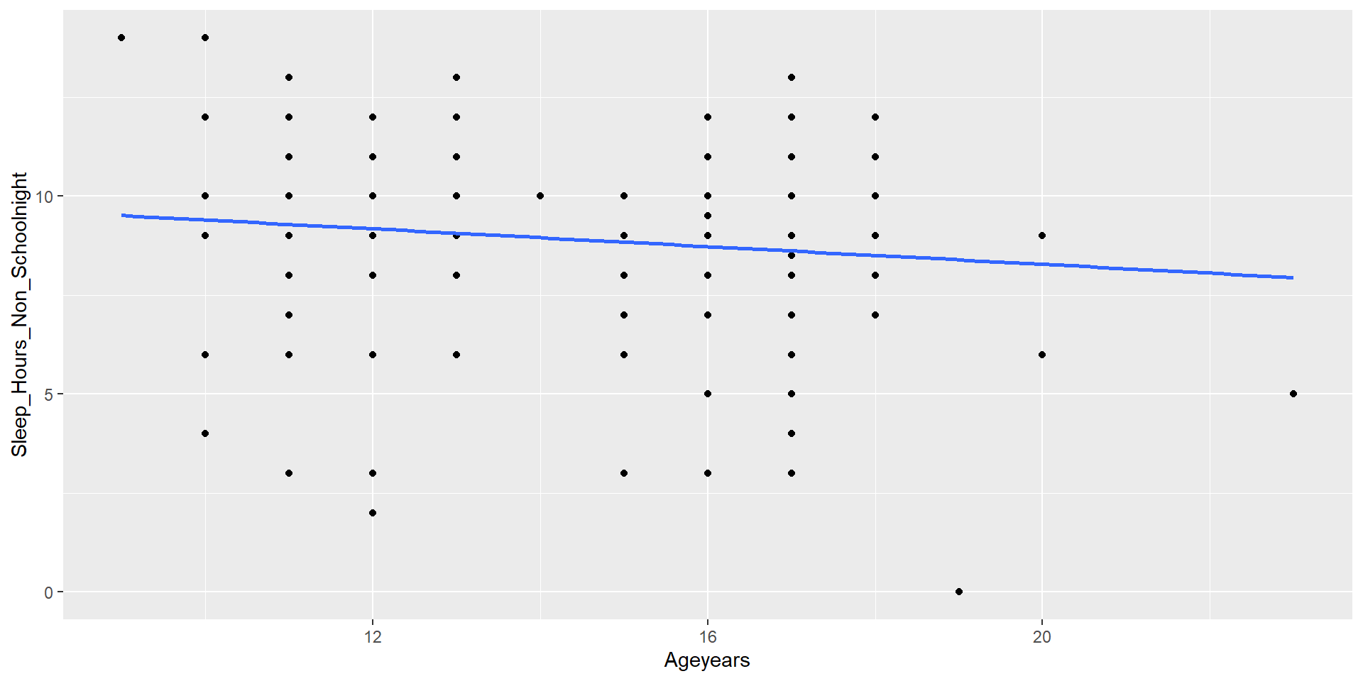
Call:
lm(formula = Sleep_Hours_Non_Schoolnight ~ Ageyears, data = school)

Residuals:
    Min      1Q  Median      3Q     Max 
-8.3947 -0.7306  0.3813  1.2694  4.5974 

Coefficients:
            Estimate Std. Error t value            Pr(>|t|)    
(Intercept) 10.52256    0.90536  11.623 <0.0000000000000002 ***
Ageyears    -0.11199    0.05887  -1.902              0.0585 .  
---
Signif. codes:  0 '***' 0.001 '**' 0.01 '*' 0.05 '.' 0.1 ' ' 1

Residual standard error: 2.204 on 204 degrees of freedom
  (1 observation deleted due to missingness)
Multiple R-squared:  0.01743,   Adjusted R-squared:  0.01261 
F-statistic: 3.619 on 1 and 204 DF,  p-value: 0.05854

summary(fit.1)$r.squared

[1] 0.01742975

r2(fit.1)

# R2 for Linear Regression
       R2: 0.017
  adj. R2: 0.013

Example

school %>% 
  ggplot(aes(x = Ageyears, y = Sleep_Hours_Non_Schoolnight)) + 
  geom_point() + geom_smooth(method = "lm", se = F)

Example - `easystats`

predicted_f1 <- estimate_expectation(fit.1, data = "grid")
plot(predicted_f1)

Example - `easystats` Check_model

check_model(fit.1)

model_performance(fit.1)

# Indices of model performance

AIC     |    AICc |     BIC |    R2 | R2 (adj.) |  RMSE | Sigma
---------------------------------------------------------------
914.120 | 914.238 | 924.103 | 0.017 |     0.013 | 2.193 | 2.204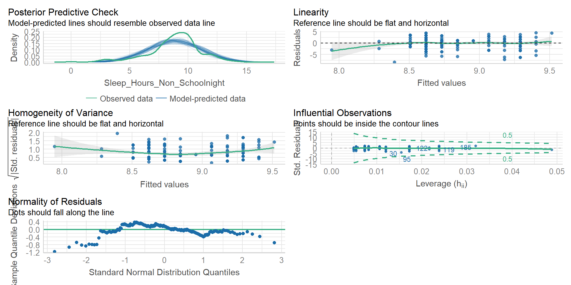

Inferential tests

NHST is about making decisions:

these two means are/are not different
this correlation is/is not significant
the distribution of this categorical variable is/is not different between these groups

In regression, there are several inferential tests being conducted at once. The first is called the omnibus test – this is a test of whether the model fits the data.

Omnibus test

Historically we use the F distribution to estimate the significance of our model, because it works with our ability to partition variance.

What is our null hypothesis?

. . .

The model does not account for variance in \(Y\) (spoiler…ANOVA)

F Distributions and regression

F statistics are not testing the likelihood of differences; they test the likelihood of ratios. In this case, we want to determine whether the variance explained by our model is larger in magnitude than another variance.

Which variance?

\[\Large F_{\nu_1\nu_2} = \frac{\frac{\chi^2_{\nu_1}}{\nu_1}}{\frac{\chi^2_{\nu_2}}{\nu_2}}\]

\[\Large F_{\nu_1\nu_2} = \frac{\frac{\text{Variance}_{\text{Model}}}{\nu_1}}{\frac{\text{Variance}_{\text{Residual}}}{\nu_2}}\]

\[\Large F = \frac{MS_{Model}}{MS_{residual}}\]

The degrees of freedom for our model are

\[DF_1 = k\] \[DF_2 = N-k-1\]

Where k is the number of IV’s in your model, and N is the sample size.

Mean squares are calculated by taking the relevant Sums of Squares and dividing by their respective degrees of freedom.

\(SS_{\text{Model}}\) is divided by \(DF_1\)
\(SS_{\text{Residual}}\) is divided by \(DF_2\)

anova(fit.1)

Analysis of Variance Table

Response: Sleep_Hours_Non_Schoolnight
           Df Sum Sq Mean Sq F value  Pr(>F)  
Ageyears    1  17.57 17.5728  3.6187 0.05854 .
Residuals 204 990.64  4.8561                  
---
Signif. codes:  0 '***' 0.001 '**' 0.01 '*' 0.05 '.' 0.1 ' ' 1

summary(fit.1)


Call:
lm(formula = Sleep_Hours_Non_Schoolnight ~ Ageyears, data = school)

Residuals:
    Min      1Q  Median      3Q     Max 
-8.3947 -0.7306  0.3813  1.2694  4.5974 

Coefficients:
            Estimate Std. Error t value            Pr(>|t|)    
(Intercept) 10.52256    0.90536  11.623 <0.0000000000000002 ***
Ageyears    -0.11199    0.05887  -1.902              0.0585 .  
---
Signif. codes:  0 '***' 0.001 '**' 0.01 '*' 0.05 '.' 0.1 ' ' 1

Residual standard error: 2.204 on 204 degrees of freedom
  (1 observation deleted due to missingness)
Multiple R-squared:  0.01743,   Adjusted R-squared:  0.01261 
F-statistic: 3.619 on 1 and 204 DF,  p-value: 0.05854

Mean square error (MSE)

AKAmean square residual and mean square within
unbiased estimate of error variance
- measure of discrepancy between the data and the model
the MSE is the variance around the fitted regression line
Note: it is a transformation of the standard error of the estimate (and residual standard error)!

Multiple Regression

Regression Equation

Going from this:

\[ \hat{Y} = b_0 + b_1X1 \]

To this

\[ \hat{Y} = b_0 + b_1X_1 + b_2X_2 + ... + b_kX_k \]

Regression coefficient values are now “partial” - Represents the contribution to all of outcome (\(\hat{Y}\)) from unique aspects of each \(X\)

Interpreting Coefficients

\[ \hat{Y} = b_0 + b_1X_1 + b_2X_2 + ... + b_kX_k \]

Focus on a specific predictor (e.g., \(X_1\))
For every 1 unit change in \(X_1\), there is a \(b_1\) unit change in \(Y\), holding all other predictors constant

Note: Properties of OLS still hold true

The sum of residuals will be 0
Each predictor (\(X\)) will be uncorrelated with the residuals

Example - Multiple Predictors

Let’s include another variable into our model to predict sleep

fit.2 <- lm(Sleep_Hours_Non_Schoolnight ~ Ageyears + video_game_hrs + social_med_hrs, 
           data = school)
summary(fit.2)


Call:
lm(formula = Sleep_Hours_Non_Schoolnight ~ Ageyears + video_game_hrs + 
    social_med_hrs, data = school)

Residuals:
    Min      1Q  Median      3Q     Max 
-8.5121 -0.7395  0.3097  1.3249  4.6458 

Coefficients:
                 Estimate Std. Error t value            Pr(>|t|)    
(Intercept)    10.1267351  0.9845471  10.286 <0.0000000000000002 ***
Ageyears       -0.0853584  0.0632637  -1.349               0.179    
video_game_hrs  0.0005255  0.0111080   0.047               0.962    
social_med_hrs -0.0042958  0.0018007  -2.386               0.018 *  
---
Signif. codes:  0 '***' 0.001 '**' 0.01 '*' 0.05 '.' 0.1 ' ' 1

Residual standard error: 2.179 on 189 degrees of freedom
  (14 observations deleted due to missingness)
Multiple R-squared:  0.03541,   Adjusted R-squared:  0.0201 
F-statistic: 2.313 on 3 and 189 DF,  p-value: 0.07744

Example - Coefficient interpretation

sjPlot

sjPlot::tab_model(fit.2)

	Sleep Hours Non Schoolnight
Predictors	Estimates	CI	p
(Intercept)	10.13	8.18 – 12.07	<0.001
Ageyears	-0.09	-0.21 – 0.04	0.179
video game hrs	0.00	-0.02 – 0.02	0.962
social med hrs	-0.00	-0.01 – -0.00	0.018
Observations	193
R² / R² adjusted	0.035 / 0.020

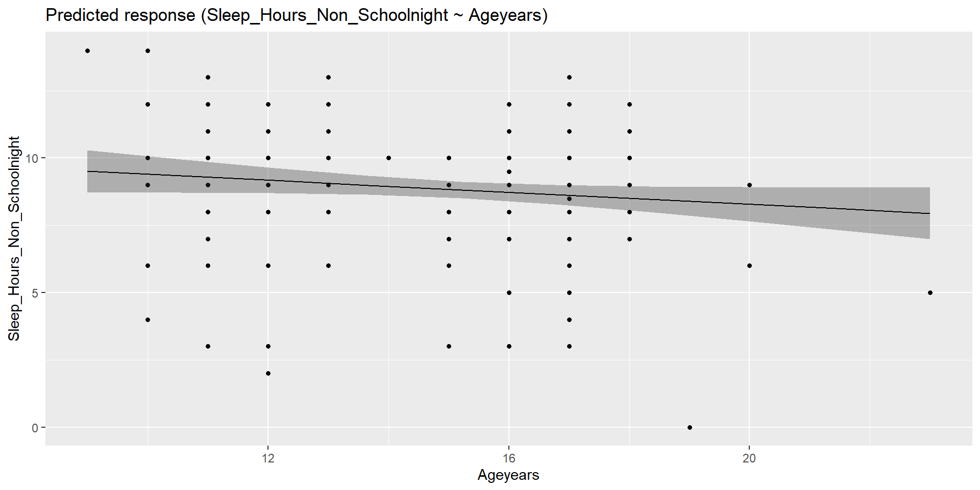
Example - Visualizing

How do we visualize this?

Example - Visualizing

How do we visualize this?

car::avPlots(fit.2)

Holding Constant??? Wut

summary(fit.2)

...
Coefficients:
                 Estimate Std. Error t value            Pr(>|t|)    
(Intercept)    10.1267351  0.9845471  10.286 <0.0000000000000002 ***
Ageyears       -0.0853584  0.0632637  -1.349               0.179    
video_game_hrs  0.0005255  0.0111080   0.047               0.962    
social_med_hrs -0.0042958  0.0018007  -2.386               0.018 *  
...

The average amount of sleep decreases by 0.08 hours for every 1 year older the youth his holding the number of hours playing video games and the number of hours on social media constant.
The average amount of sleep decreases by 0.004 hours for every 1 hour of social media use holding age and hours of video game usage constant.

What does this mean?? Also can be called “controlling for” or “taking into account” the other variables

Language comes from experimental research in which they can keep one condition unchanged while manipulating the other

Holding Constant - “Controlling for”

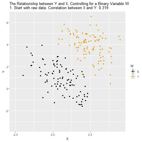
Taken from @nickchk

Creating the Model

There can be many different ways in which we create and compare models with multiple predictors

Simultaneous: Enter all variables in the model at once
- Usually the most conservative and defensible approach (unless there is theory to support a hierarchical approach)
Hierarchically: Building a sequence of models where a single variable is included/excluded at each step
- This is hierarchical/stepwise regression. Different from HLM (Hierarchical Linear Modeling)

Model Selection (LSR 15.10)

How can we tell if one model is “better” than the other (it explains more variance in outcome)?

Each predictor (or set of predictors) is investigated as to what it adds to the model when it is entered
The order of the variables depends on an a priori hypothesis

The concept is to ask how much variance is unexplained by our model. The leftovers can be compared to an alternate model to see if the new variable adds anything or if we should focus on parsimony

Model Comparison Example

m.2 <- lm(Sleep_Hours_Non_Schoolnight ~ Ageyears + video_game_hrs, 
           data = school)
m.3 <- lm(Sleep_Hours_Non_Schoolnight ~ Ageyears + video_game_hrs + social_med_hrs, 
           data = school)
anova(m.2, m.3)

...
Analysis of Variance Table

Model 1: Sleep_Hours_Non_Schoolnight ~ Ageyears + video_game_hrs
Model 2: Sleep_Hours_Non_Schoolnight ~ Ageyears + video_game_hrs + social_med_hrs
  Res.Df    RSS Df Sum of Sq      F  Pr(>F)  
1    190 924.10                              
2    189 897.09  1    27.014 5.6912 0.01804 *
...

r2(m.2)

# R2 for Linear Regression
       R2: 0.006
  adj. R2: -0.004

r2(m.3)

# R2 for Linear Regression
       R2: 0.035
  adj. R2: 0.020

Model Comparison - sjPlot

tab_model(m.2, m.3)

	Sleep Hours Non Schoolnight			Sleep Hours Non Schoolnight
Predictors	Estimates	CI	p	Estimates	CI	p
(Intercept)	9.81	7.86 – 11.76	<0.001	10.13	8.18 – 12.07	<0.001
Ageyears	-0.07	-0.20 – 0.06	0.274	-0.09	-0.21 – 0.04	0.179
video game hrs	-0.00	-0.02 – 0.02	0.949	0.00	-0.02 – 0.02	0.962
social med hrs				-0.00	-0.01 – -0.00	0.018
Observations	193			193
R² / R² adjusted	0.006 / -0.004			0.035 / 0.020

Model Diagnostics

Checking the model (LSR 15.9)

Whenever we are looking at the regression model diagnostics, we are often considering the residual values. The types of residuals we can look at are:

Ordinary Residuals - Raw
Standardized Residuals
Studentized Residuals - Takes into account what the SD would have been with the removal of the \(i\)th observation

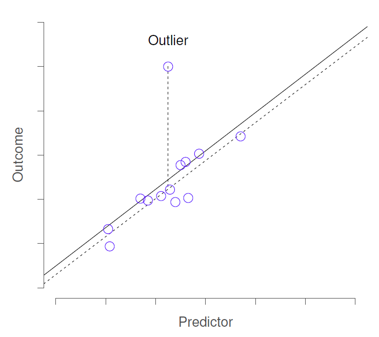
Model Checks - Outlier

We tend to look for various things that may impact our results through the lens of residuals

1) Outliers - variables with high Studentized Residuals

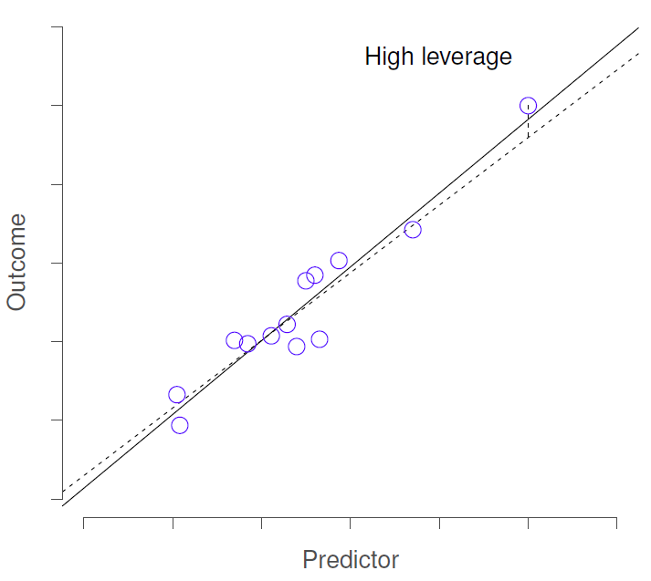
Model Checks - Leverage

We tend to look for various things that may impact our results through the lens of residuals

2) Leverage - variable is different in all ways from others (not just residuals)

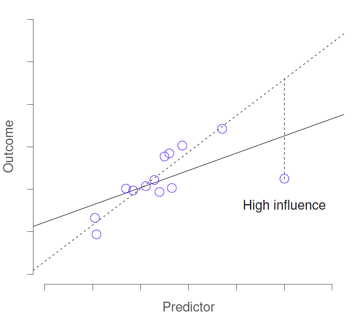
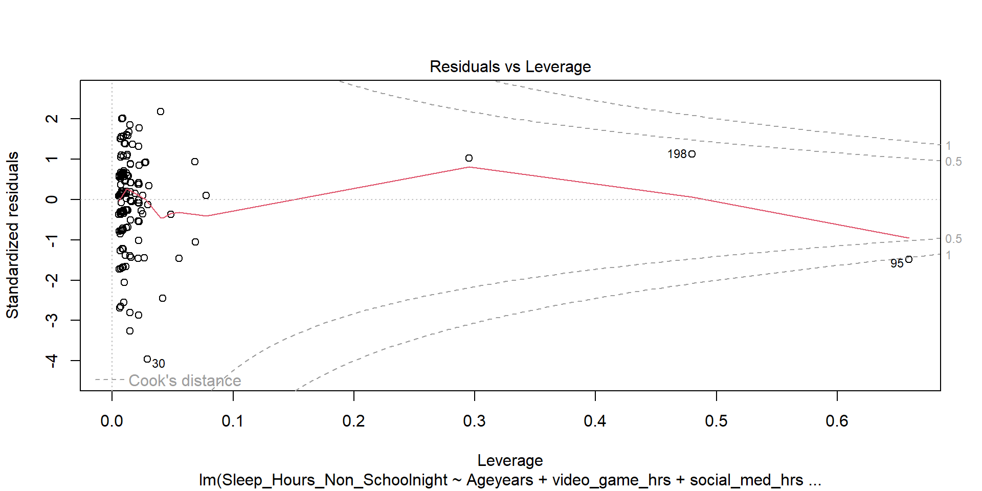
Model Checks - Influence

We tend to look for various things that may impact our results through the lens of residuals

3) Influence - outlier with high leverage (Cook’s Distance)

Model Checks - Plots

#Cook's Distance
plot(m.3, which = 4)

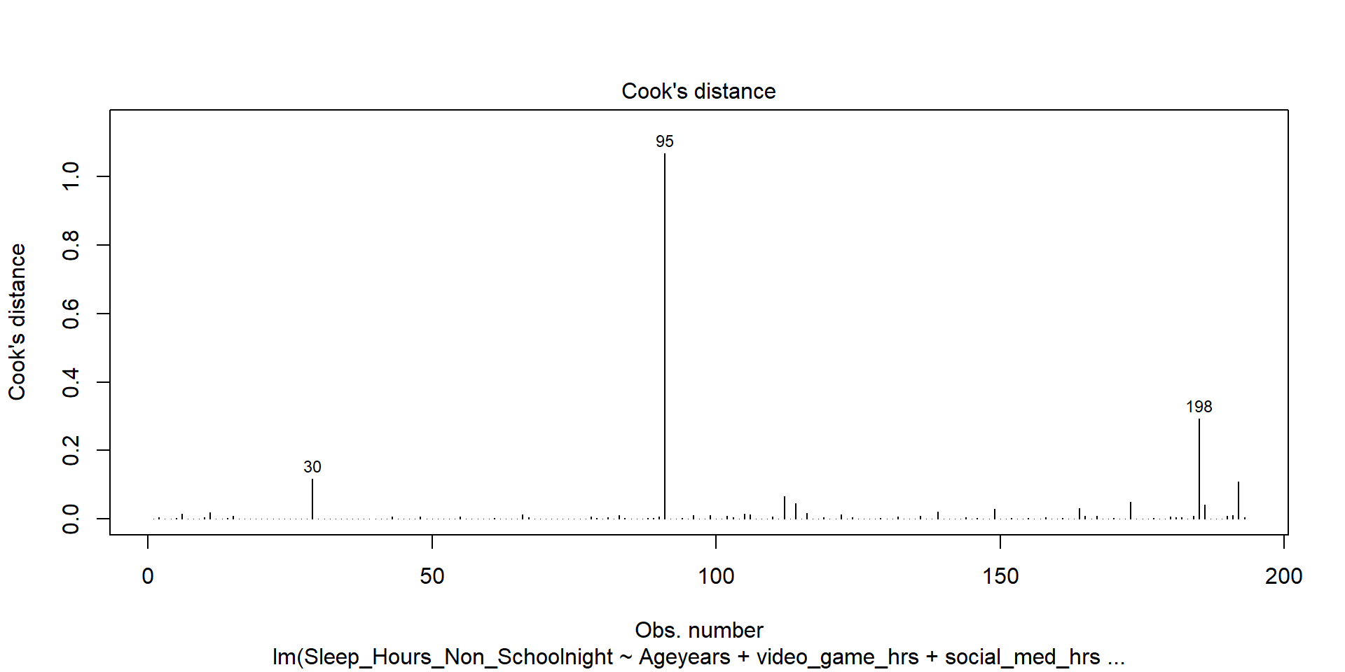
Model Checks - Plots

#Leverage
plot(m.3, which = 5)

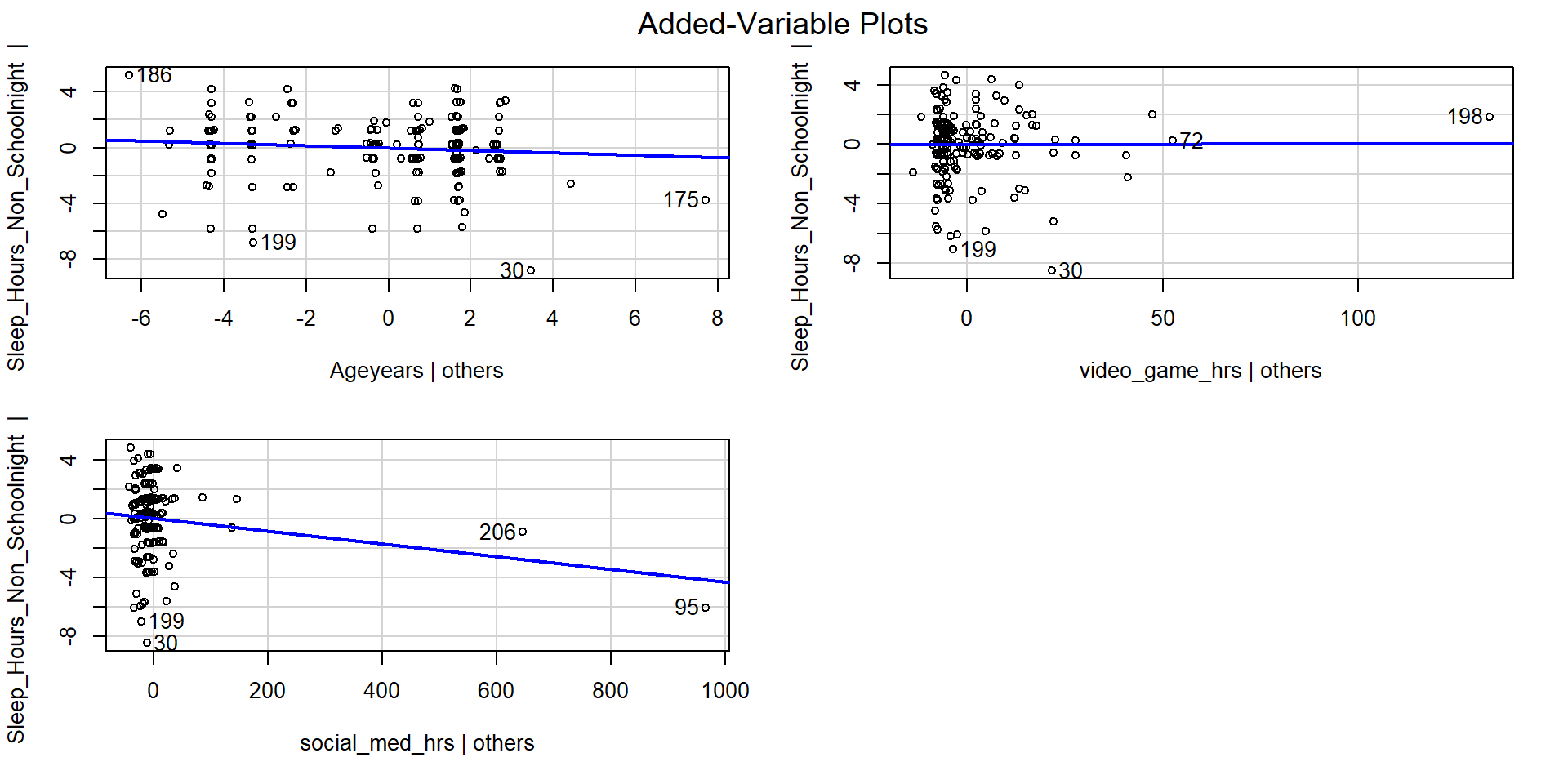
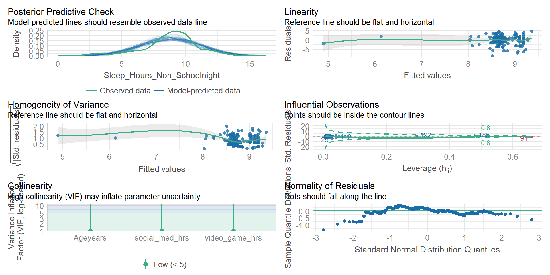
Checking Collinearity

We need to check to see if our predictor variables are too highly correlated with each other

To do so we use variance inflation factors (VIF)

There will be a VIF that is associated with each predictor in the model
Interpreting VIF (link) - Starts at 1 and goes up
- 1 = Not Correlated
- 1-5 = Moderately Correlated
- 5+ = Highly Correlated

car::vif(m.3)

      Ageyears video_game_hrs social_med_hrs 
      1.012331       1.003960       1.012351

`easystats` making stats easy

Can check the model with a simple function

check_model(m.3)

Rounding up Multiple Regression

It is a powerful and complex tool

Next time…

More R fun
Group work

Multiple Regression: A story of betas

Last Time

Today…

Data for Today

Example

Example

Example - easystats

Example - easystats Check_model

Inferential tests

Omnibus test

F Distributions and regression

Mean square error (MSE)

Multiple Regression

Regression Equation

Interpreting Coefficients

Example - Multiple Predictors

Example - Coefficient interpretation

Example - Visualizing

Example - Visualizing

Holding Constant??? Wut

Holding Constant - “Controlling for”

Creating the Model

Model Selection (LSR 15.10)

Model Comparison Example

Model Comparison - sjPlot

Model Diagnostics

Checking the model (LSR 15.9)

Model Checks - Outlier

Model Checks - Leverage

Model Checks - Influence

Model Checks - Plots

Model Checks - Plots

Checking Collinearity

easystats making stats easy

Rounding up Multiple Regression

Next time…

Stop…Group Time

Example - `easystats`

Example - `easystats` Check_model

`easystats` making stats easy