Intro to RMarkdown (and some regression stuff)

PSYC 640 - Fall 2023

Dustin Haraden, PhD

Overview

Next couple of classes will be split between group work and R Markdown fancifulness

Presentations will start on Wednesday 12/6

Peer Review of Data analytic plan will be assigned tomorrow (how quickly can this be done?)

What are other things we can do? Or questions you have?

Last Time

Multiple Regression
Group work stuff

Today…

Review the regression stuff
RMarkdown!
- Even though we’ve been doing it this whole time

options(scipen=999)
library(car) #recode conflict with tidyverse
library(tidyverse)
library(psych)
library(easystats)
library(sjPlot)
library(janitor)

Data for Today

student_perf <- read_csv("https://raw.githubusercontent.com/dharaden/psyc640/main/data/Multiple_reg/Student_Performance.csv") %>% 
  clean_names()

This data is taken from Kaggle and is simulated data to explore multiple linear regression. Variables include:

Scores from previous test
Average sleep hours
Average hours studied

Participating in Extracurriculars
# of Practice Questions used
Performance Index (Outcome)

Multiple Regression

Regression Equation

Going from this:

\[ \hat{Y} = b_0 + b_1X1 \]

To this

\[ \hat{Y} = b_0 + b_1X_1 + b_2X_2 + ... + b_kX_k \]

Regression coefficient values are now “partial” - Represents the contribution to all of outcome (\(\hat{Y}\)) from unique aspects of each \(X\)

Example - Single Predictor (`tab_model()`)

Can customize the tables which we will focus more on in the next section

fit1 <- lm(performance_index ~ hours_studied, 
           data = student_perf)

summary(fit1)


Call:
lm(formula = performance_index ~ hours_studied, data = student_perf)

Residuals:
    Min      1Q  Median      3Q     Max 
-33.667 -14.093   0.226  15.205  33.226 

Coefficients:
              Estimate Std. Error t value             Pr(>|t|)    
(Intercept)     39.646      2.659  14.912 < 0.0000000000000002 ***
hours_studied    3.128      0.464   6.741       0.000000000157 ***
---
Signif. codes:  0 '***' 0.001 '**' 0.01 '*' 0.05 '.' 0.1 ' ' 1

Residual standard error: 17.67 on 205 degrees of freedom
Multiple R-squared:  0.1814,    Adjusted R-squared:  0.1774 
F-statistic: 45.43 on 1 and 205 DF,  p-value: 0.0000000001569

sjPlot::tab_model(fit1, show.std = TRUE, 
                  title = "Figure 1", 
                  pred.labels = c("Int.", "Hours Studied"), 
                  dv.labels = "Performance Index")

Figure 1
	Performance Index
Predictors	Estimates	std. Beta	CI	standardized CI	p
Int.	39.65	-0.00	34.40 – 44.89	-0.12 – 0.12	<0.001
Hours Studied	3.13	0.43	2.21 – 4.04	0.30 – 0.55	<0.001
Observations	207
R² / R² adjusted	0.181 / 0.177

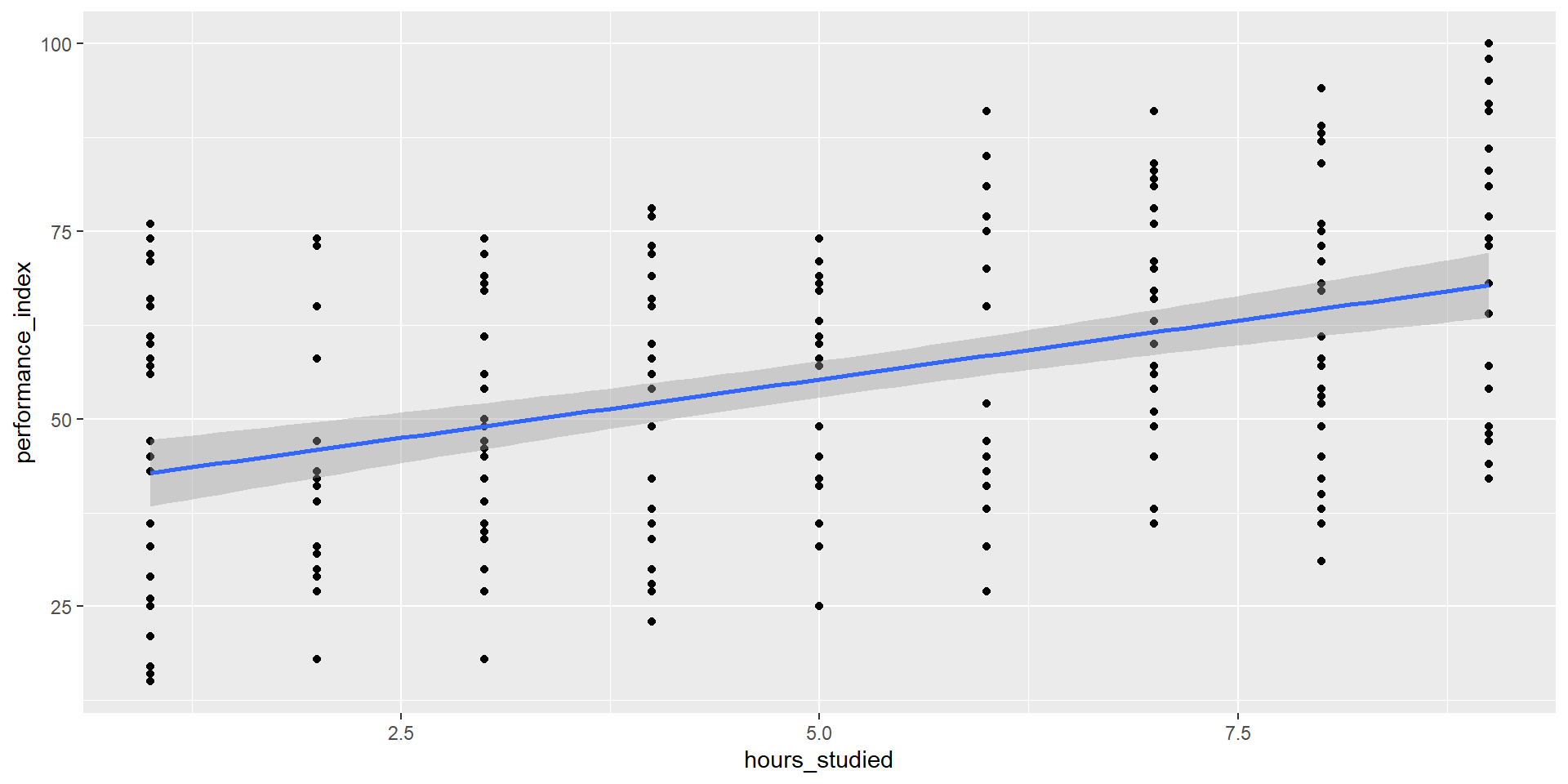
Single Predictor - Visualizing

student_perf %>% 
  ggplot(aes(x = hours_studied, 
             y = performance_index)) + 
  geom_point() + 
  geom_smooth(method = "lm")

Single Predictor- Reporting

report(fit1)

We fitted a linear model (estimated using OLS) to predict performance_index
with hours_studied (formula: performance_index ~ hours_studied). The model
explains a statistically significant and moderate proportion of variance (R2 =
0.18, F(1, 205) = 45.43, p < .001, adj. R2 = 0.18). The model's intercept,
corresponding to hours_studied = 0, is at 39.65 (95% CI [34.40, 44.89], t(205)
= 14.91, p < .001). Within this model:

  - The effect of hours studied is statistically significant and positive (beta =
3.13, 95% CI [2.21, 4.04], t(205) = 6.74, p < .001; Std. beta = 0.43, 95% CI
[0.30, 0.55])

Standardized parameters were obtained by fitting the model on a standardized
version of the dataset. 95% Confidence Intervals (CIs) and p-values were
computed using a Wald t-distribution approximation.

Multiple Predictors - Example

Now let’s add in some other variables that we think may contribute to a student’s “Performance Index”

fit2 <- lm(performance_index ~ hours_studied + sleep_hours + previous_scores, 
           data = student_perf)

summary(fit2)


Call:
lm(formula = performance_index ~ hours_studied + sleep_hours + 
    previous_scores, data = student_perf)

Residuals:
    Min      1Q  Median      3Q     Max 
-5.3665 -1.3541 -0.0376  1.3853  4.5946 

Coefficients:
                  Estimate Std. Error t value             Pr(>|t|)    
(Intercept)     -33.159893   0.805496 -41.167 < 0.0000000000000002 ***
hours_studied     2.853131   0.052487  54.359 < 0.0000000000000002 ***
sleep_hours       0.436876   0.077699   5.623         0.0000000617 ***
previous_scores   1.022061   0.008128 125.749 < 0.0000000000000002 ***
---
Signif. codes:  0 '***' 0.001 '**' 0.01 '*' 0.05 '.' 0.1 ' ' 1

Residual standard error: 1.995 on 203 degrees of freedom
Multiple R-squared:  0.9897,    Adjusted R-squared:  0.9895 
F-statistic:  6480 on 3 and 203 DF,  p-value: < 0.00000000000000022

Interpreting Coefficients

\[ \hat{Y} = b_0 + b_1X_1 + b_2X_2 + ... + b_kX_k \]

Focus on a specific predictor (e.g., \(X_1\))
For every 1 unit change in \(X_1\), there is a \(b_1\) unit change in \(Y\), holding all other predictors constant

Note: Properties of OLS still hold true

The sum of residuals will be 0
Each predictor (\(X\)) will be uncorrelated with the residuals

Holding Constant??? Wut

tab_model(fit2)

	performance index
Predictors	Estimates	CI	p
(Intercept)	-33.16	-34.75 – -31.57	<0.001
hours studied	2.85	2.75 – 2.96	<0.001
sleep hours	0.44	0.28 – 0.59	<0.001
previous scores	1.02	1.01 – 1.04	<0.001
Observations	207
R² / R² adjusted	0.990 / 0.990

Reporting the results

report(fit2)

We fitted a linear model (estimated using OLS) to predict performance_index
with hours_studied, sleep_hours and previous_scores (formula: performance_index
~ hours_studied + sleep_hours + previous_scores). The model explains a
statistically significant and substantial proportion of variance (R2 = 0.99,
F(3, 203) = 6479.94, p < .001, adj. R2 = 0.99). The model's intercept,
corresponding to hours_studied = 0, sleep_hours = 0 and previous_scores = 0, is
at -33.16 (95% CI [-34.75, -31.57], t(203) = -41.17, p < .001). Within this
model:

  - The effect of hours studied is statistically significant and positive (beta =
2.85, 95% CI [2.75, 2.96], t(203) = 54.36, p < .001; Std. beta = 0.39, 95% CI
[0.37, 0.40])
  - The effect of sleep hours is statistically significant and positive (beta =
0.44, 95% CI [0.28, 0.59], t(203) = 5.62, p < .001; Std. beta = 0.04, 95% CI
[0.03, 0.05])
  - The effect of previous scores is statistically significant and positive (beta
= 1.02, 95% CI [1.01, 1.04], t(203) = 125.75, p < .001; Std. beta = 0.90, 95%
CI [0.88, 0.91])

Standardized parameters were obtained by fitting the model on a standardized
version of the dataset. 95% Confidence Intervals (CIs) and p-values were
computed using a Wald t-distribution approximation.

Creating the Model

There can be many different ways in which we create and compare models with multiple predictors

Simultaneous: Enter all variables in the model at once
- Usually the most conservative and defensible approach (unless there is theory to support a hierarchical approach)
Hierarchically: Building a sequence of models where a single variable is included/excluded at each step
- This is hierarchical/stepwise regression. Different from HLM (Hierarchical Linear Modeling)

Model Selection (LSR 15.10)

How can we tell if one model is “better” than the other (it explains more variance in outcome)?

Each predictor (or set of predictors) is investigated as to what it adds to the model when it is entered
The order of the variables depends on an a priori hypothesis

The concept is to ask how much variance is unexplained by our model. The leftovers can be compared to an alternate model to see if the new variable adds anything or if we should focus on parsimony

Model Diagnostics

Checking the model (LSR 15.9)

Whenever we are looking at the regression model diagnostics, we are often considering the residual values. The types of residuals we can look at are:

Ordinary Residuals - Raw
Standardized Residuals
Studentized Residuals - Takes into account what the SD would have been with the removal of the \(i\)th observation

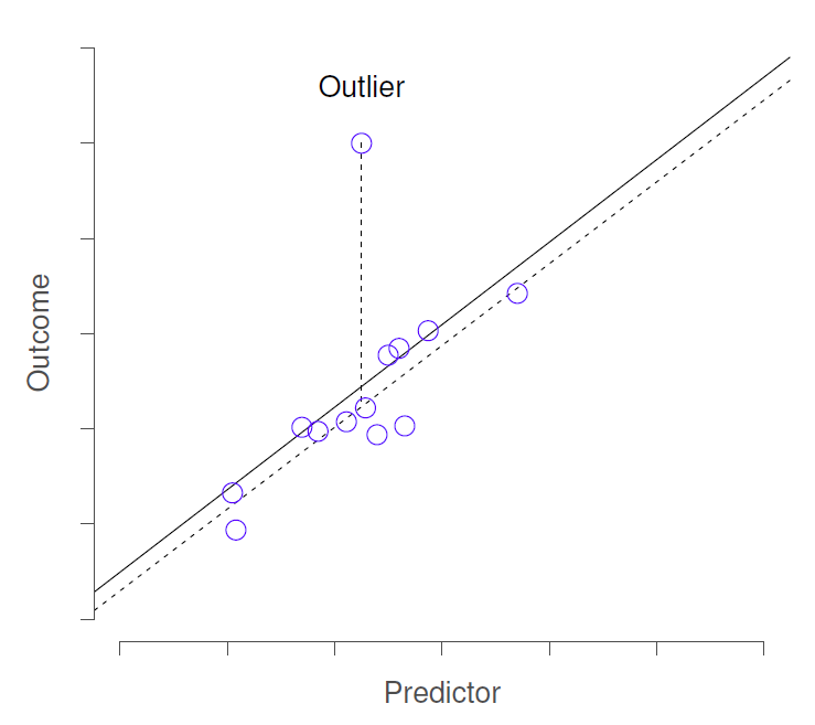
Model Checks - Outlier

We tend to look for various things that may impact our results through the lens of residuals

1) Outliers - variables with high Studentized Residuals

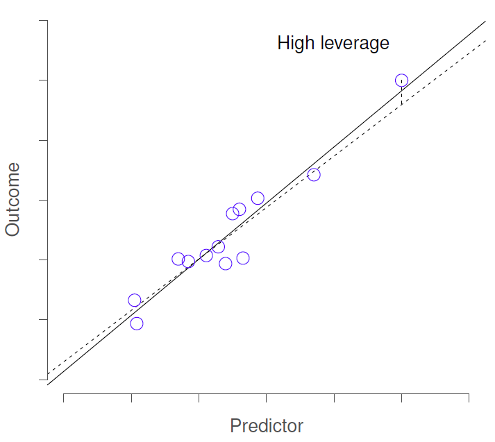
Model Checks - Leverage

We tend to look for various things that may impact our results through the lens of residuals

2) Leverage - variable is different in all ways from others (not just residuals)

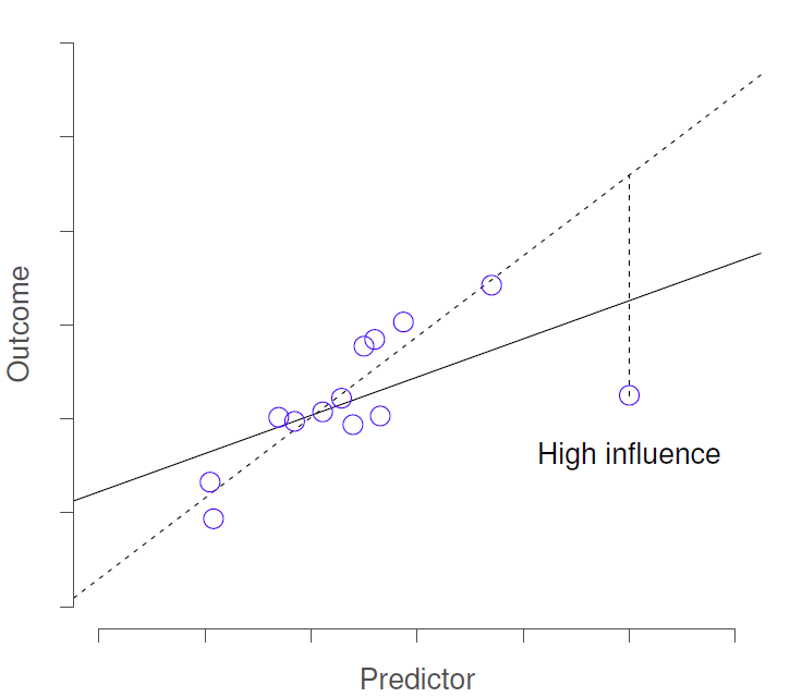
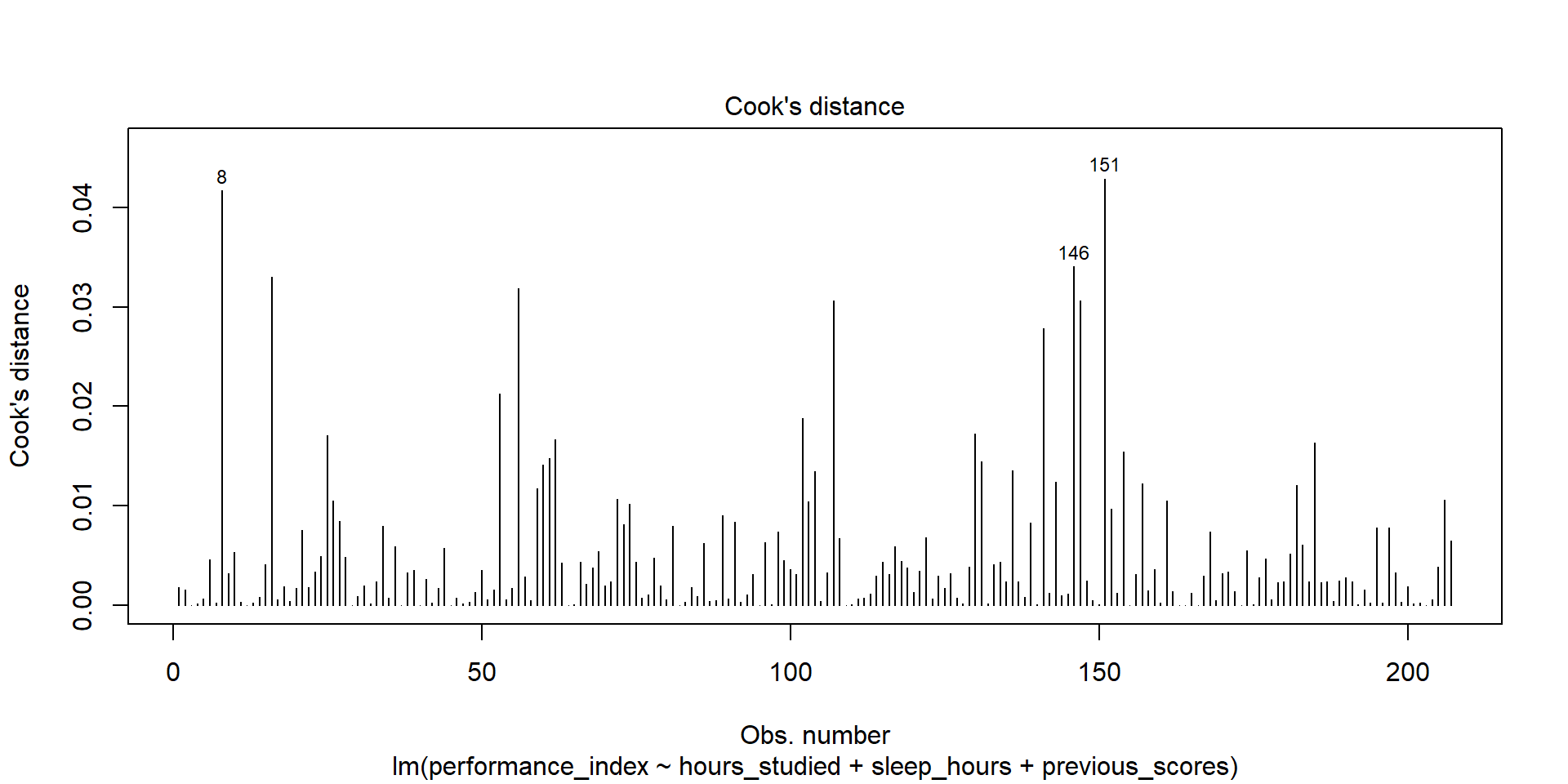
Model Checks - Influence

We tend to look for various things that may impact our results through the lens of residuals

3) Influence - outlier with high leverage (Cook’s Distance)

Model Checks - Plots

#Cook's Distance
plot(fit2, which = 4)

Checking Collinearity

We need to check to see if our predictor variables are too highly correlated with each other

To do so we use variance inflation factors (VIF)

There will be a VIF that is associated with each predictor in the model
Interpreting VIF (link) - Starts at 1 and goes up
- 1 = Not Correlated
- 1-5 = Moderately Correlated
- 5+ = Highly Correlated

car::vif(fit2)

  hours_studied     sleep_hours previous_scores 
       1.003645        1.002031        1.002236

RMarkdown

This is something that we have been using this whole time!

The script that we use allows us to embed both regular text and code all into a single document. This is what we use for the labs with various levels of success when it comes to knitting the document

We’ll be spending more time exploring all the cool things that RMarkdown can do

Some Useful Resources

R Markdown: The Definitive Guide

R Markdown Cheatsheet

R Markdown Cookbook

Custom Formats for R Markdown

Ideas for topics to Highlight

Making sure we can have things knit
HTML Templates
Code Chunk Options (Cheatsheet)
Fun things to do with HTML Output

Intro to RMarkdown (and some regression stuff)

Overview

Last Time

Today…

Data for Today

Multiple Regression

Regression Equation

Example - Single Predictor (tab_model())

Single Predictor - Visualizing

Single Predictor- Reporting

Multiple Predictors - Example

Interpreting Coefficients

Holding Constant??? Wut

Reporting the results

Creating the Model

Model Selection (LSR 15.10)

Model Diagnostics

Checking the model (LSR 15.9)

Model Checks - Outlier

Model Checks - Leverage

Model Checks - Influence

Model Checks - Plots

Checking Collinearity

RMarkdown

RMarkdown

Some Useful Resources

Ideas for topics to Highlight

Example - Single Predictor (`tab_model()`)