Determine the sampling distribution (will be using \(F\)-distribution now)
Identify the critical value
Calculate test statistic for sample collected
Inspect & compare statistic to critical value; Calculate probability
Steps to calculating F-ratio
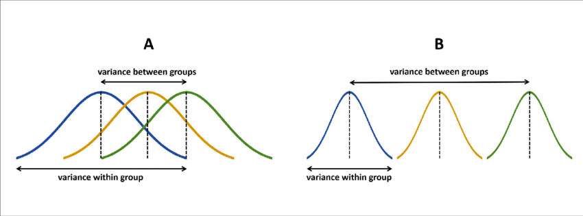
Variance to Sum of Squares (Between & Within)
Degrees of Freedom
Mean squares values
F-Statistic
Calculating the F-Statistic
\[F = \frac{MS_b}{MS_w}\]
If the null hypothesis is true, \(F\) has an expected value close to 1 (numerator and denominator are estimates of the same variability)
If it is false, the numerator will likely be larger, because systematic, between-group differences contribute to the variance of the means, but not to variance within group.
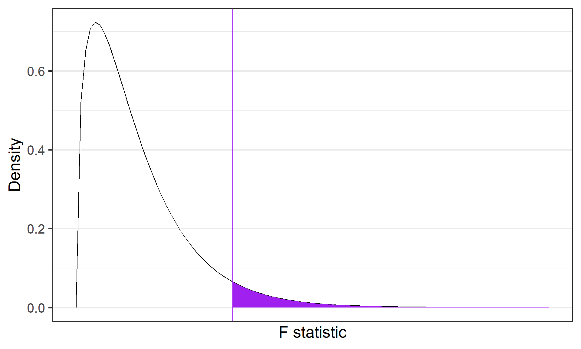
If data are normally distributed, then the variance is \(\chi^2\) distributed
\(F\)-distributions are one-tailed tests. Recall that we’re interested in how far away our test statistic from the null \((F = 1).\)
ANOVA table
Source of Variation
df
Sum of Squares
Mean Squares
F-statistic
p-value
Group
\(G-1\)
\(SS_b\)
\(MS_b = \frac{SS_b}{df_b}\)
\(F = \frac{MS_b}{MS_w}\)
\(p\)
Residual
\(N-G\)
\(SS_w\)
\(MS_w = \frac{SS_w}{df_w}\)
Total
\(N-1\)
\(SS_{total}\)
Contrasts/Post-Hoc
Contrasts/Post-Hoc Tests
Performed when there is a significant difference among the groups to examine which groups are different
Contrasts: When we have a priori hypotheses
Post-hoc Tests: When we want to test everything
These comparisons take the general form of t-tests, but note some extensions:
the pooled variance estimate comes from \(SS_{\text{residual}}\), meaning it pulls information from all groups
the degrees of freedom for the \(t\)-test is \(N-k\), so using all data
Previous Spooky Data
EMF rating across multiple locations
spooky <-import("https://raw.githubusercontent.com/dharaden/dharaden.github.io/main/data/SS%20Calculations.csv") %>%select(Location, EMF) #There were some extra empty variables in there that we don't care aboutfit_1 <-aov(EMF ~ Location, data = spooky)summary(fit_1)
             Df Sum Sq Mean Sq F value              Pr(>F)
Location      7   5115   730.7   523.5 <0.0000000000000002 ***
Residuals   138    193     1.4
---
Signif. codes:  0 '***' 0.001 '**' 0.01 '*' 0.05 '.' 0.1 ' ' 1
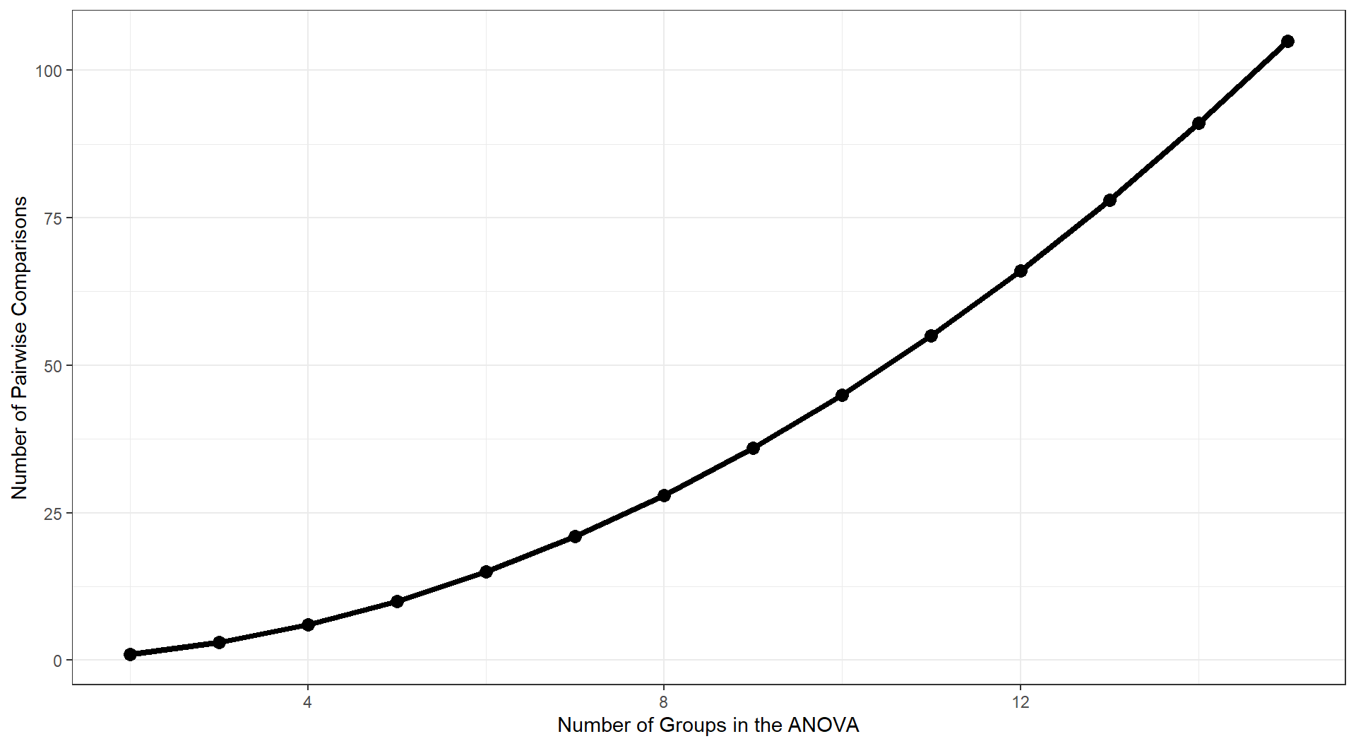
These pairwise comparisons can quickly grow in number as the number of Groups increases. With 8 (k) Groups, we have k(k-1)/2 = 28 possible pairwise comparisons.
As the number of groups in the ANOVA grows, the number of possible pairwise comparisons increases dramatically.
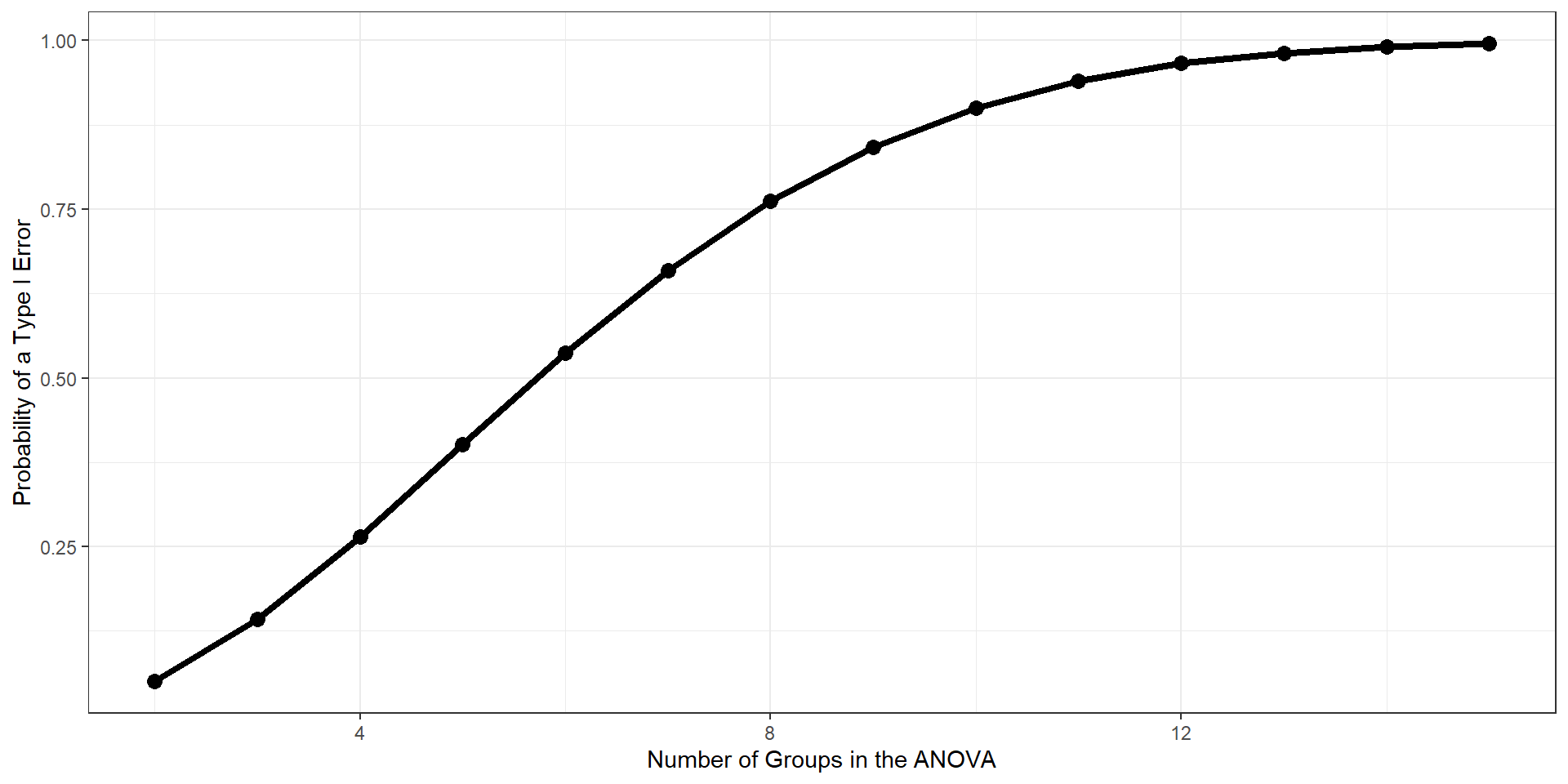
As the number of tests grows, and assuming the null hypothesis is true, the probability that we will make one or more Type I errors increases. To approximate the magnitude of the problem, we can assume that the multiple pairwise comparisons are independent. The probability that we don’t make a Type I error for one test is:
\[P(\text{No Type I}, 1 \text{ test}) = 1-\alpha\]
The probability that we don’t make a Type I error for two tests is:
\[P(\text{No Type I}, 2 \text{ test}) = (1-\alpha)(1-\alpha)\]
For C tests, the probability that we make no Type I errors is
\[P(\text{No Type I}, C \text{ tests}) = (1-\alpha)^C\]
We can then use the following to calculate the probability that we make one or more Type I errors in a collection of C independent tests.
\[P(\text{At least one Type I}, C \text{ tests}) = 1-(1-\alpha)^C\]
The Type I error inflation that accompanies multiple comparisons motivates the large number of “correction” procedures that have been developed.
Multiple comparisons, each tested with \(\alpha_{per-test}\), increases the family-wise \(\alpha\) level.
\[\large \alpha_{family-wise} = 1 - (1-\alpha_{per-test})^C\] Šidák showed that the family-wise a could be controlled to a desired level (e.g., .05) by changing the \(\alpha_{per-test}\) to:
The Bonferroni procedure is conservative. Other correction procedures have been developed that control family-wise Type I error at .05 but that are more powerful than the Bonferroni procedure. The most common one is the Holm procedure.
The Holm procedure does not make a constant adjustment to each per-test \(\alpha\). Instead it makes adjustments in stages depending on the relative size of each pairwise p-value.
Holm correction
Rank order the p-values from largest to smallest.
Start with the smallest p-value. Multiply it by its rank.
Go to the next smallest p-value. Multiply it by its rank. If the result is larger than the adjusted p-value of next smallest rank, keep it. Otherwise replace with the previous step adjusted p-value.
Repeat Step 3 for the remaining p-values.
Judge significance of each new p-value against \(\alpha = .05\).
Good for 3+ groups when you have more specific hypotheses (contrasts)
Two-Way ANOVA
What is a Two-Way ANOVA?
Examines the impact of 2 nominal/categorical variables on a continuous outcome
We can now examine:
The impact of variable 1 on the outcome (Main Effect)
The impact of variable 2 on the outcome (Main Effect)
The interaction of variable 1 & 2 on the outcome (Interaction Effect)
The effect of variable 1 depends on the level of variable 2
Two-Way ANOVA: Assumptions
Same as what we’ve examined previously, plus a couple more:
Independence
Normality of Residuals
Homoscedasticity (Homogeneity of Variance)
Additivity
The effects of each factor are consistent across all levels of the other factor
Multicollinearity
Correlations between factors. This can make it difficult to separate unique contributions to the outcome
Equal Cell Sizes (N)
Main Effect & Interactions
Main Effect: Basically a one-way ANOVA
The effect of variable 1 is the same across all levels of variable 2
Interaction:
Able to examine the effect of variable 1 across different levels of variable 2
Basically speaking, the effect of variable 1 on our outcome DEPENDS on the levels of variable 2
Example Data
Data
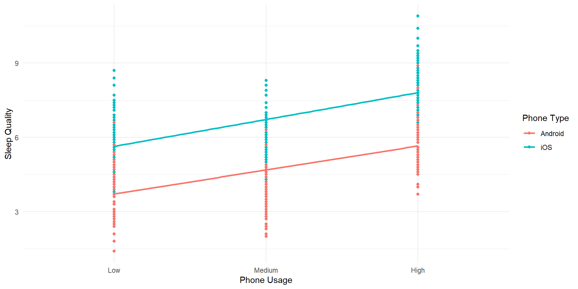
We are interested on the impact of phone usage on overall sleep quality
We include 2 variables of interest: 1) Phone Type (iOS vs. Android) and 2) Amount of usage (High, Medium & Low) to examine if there are differences in terms of sleep quality
Note: It is important to consider HOW we operationalize constructs as some things we have as factors could easily be continuous variables
Code
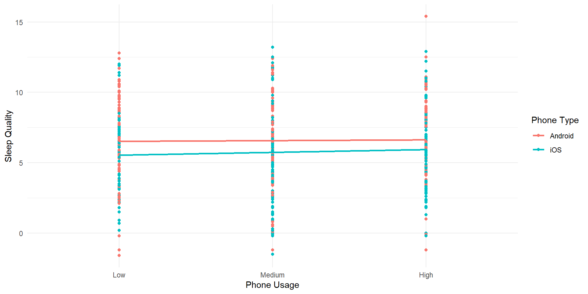
#Generate some data# Set random seed for reproducibilityset.seed(42)n <-500# Set number of observations# Generate Type of Phone dataphone_type <-sample(c("Android", "iOS"), n, replace =TRUE)# Generate Phone Usage dataphone_usage <-factor(sample(c("Low", "Medium", "High"), n, replace =TRUE), levels=c("Low", "Medium", "High"))# Generate Sleep Quality data (with some variation)# Intentionally inflating to highlight main effectssleep_quality <-round(rnorm(n, mean =ifelse(phone_type =="Android", 5, 7) +ifelse(phone_usage =="High", 1, -1), sd =1),1)# Generate Sleep Quality data (with some variation)sleep_quality2 <-round(rnorm(n, mean =6, sd =3),1)# Create a data framesleep_data <-data.frame(phone_type, phone_usage, sleep_quality, sleep_quality2)head(sleep_data)
  phone_type phone_usage sleep_quality sleep_quality2
1    Android        High           5.0           12.5
2    Android         Low           3.8           12.8
3    Android      Medium           3.9            8.7
4    Android      Medium           3.3            5.8
5        iOS         Low           5.6            8.0
6        iOS        High           7.8            3.6
Test Statistics
We’ve gone too far today without me showing some equations
With one way anova, we calculated the \(SS_{between}\) and the \(SS_{within}\) and were able to use those to capture the F-statistic
Now we have another variable to take into account. Therefore, we need to calculate:
# Create an interaction plot using ggplot2ggplot(sleep_data, aes(x = phone_usage, y = sleep_quality2, color = phone_type, group = phone_type)) +geom_point() +geom_smooth(method ="lm",se=FALSE) +labs(x ="Phone Usage", y ="Sleep Quality", color ="Phone Type") +theme_minimal()