Resources
Random Libraries
rempsych - Convenience functions for psychology
tidySEM - Provides a ‘tidy’ workflow for conducting, reporting and plotting Structural Equation Modeling
easystats - An R Framework for Easy Statistical Modeling, Visualization, and Reporting
Getting Started with R
Installing R & R-Studio
To get started with using the statistical software, we first must install it! Here is a guide that was put together to help with the installation process. Throughout this guide, you will install R followed by R-Studio (a program to make R more user friendly).
We will go over this during the first day of class, so this guide is just to use as reference.
Things needed:
Computer
Internet Connection
A coffee or preferred beverage usually helps!
R: Download and Install
Information taken from “Hands-On Programming with R”
R is maintained by an international team of developers who make the language available through the web page ofThe Comprehensive R Archive Network. The top of the web page provides three links for downloading R. Follow the link that describes your operating system: Windows or Mac.
Windows
To install R on Windows, click the “Download R for Windows” link.Then click the “base” link. Next, click the first link at the top of the new page. This link should say something like “Download R 4.3.1 for Windows,” except the 4.3.1 will be replaced by the most current version of R. The link downloads an installer program, which installs the most up-to-date version of R for Windows. Run this program and step through the installation wizard that appears. The wizard will install R into your program files folders and place a shortcut in your Start menu. Note that you’ll need to have all of the appropriate administration privileges to install new software on your machine.
Mac
To install R on a Mac, click the “Download R for Mac’’ link. Next, click on the “R-4.3.1-arm64.pkg” package link (or the package link for the most current release of R that is appropriate for your computer). An installer will download to guide you through the installation process, which is very easy. The installer lets you customize your installation, but the defaults will be suitable for most users. I’ve never found a reason to change them. If your computer requires a password before installing new programs, you’ll need it here.
Using R
R isn’t a program that you can open and start using, like Microsoft Word or Internet Explorer. Instead, R is a computer language, like C, C++, or UNIX. You use R by writing commands in the R language and asking your computer to interpret them. In the old days, people ran R code in a UNIX terminal window—as if they were hackers in a movie from the 1980s. Now almost everyone uses R with an application called RStudio, and I recommend that you do, too.
Go ahead and try to open R without using R-Studio. You will get something like this:
R-Studio: Download and Install
RStudio is an application like Microsoft Word—except that instead of helping you write in English, RStudio helps you write in R. We will use RStudio throughout because it makes working with R SO much easier. Plus there are a lot of additional functionalities that RStudio has that will expand what you can do (e.g., RMarkdown). Also, the RStudio interface looks the same for the various operating systems which will make teaching and your experience with the material a lot easier.
RStudio (the company) has recently changed their name to Posit. To download RStudio, you can navigate to the Posit download page for “RStudio Desktop”. We have already completed Step 1 (you could have just come here to download it, but it is helpful to know where to get the latest versions and materials)! All you have to do is select the box under “2: Install RStudio” to download. It should recognize the operating system that you are using, but if it does not, you will just need to scroll down the page to identify the appropriate installer.
Now you are all set and ready to go! Nice job following the instructions and getting R and RStudio on your computer. Next you can begin to customize and get used to using RStudio. Remember, this is not something that is scary or a thing you can “break”. When in doubt, check out Google or reach out to the professor!
Setting things up
Here are some things that I am going to suggest to make your experience with R as good as we possibly can. Some of the suggestions here are related to your workflow while others are direct settings within R…and some are both. We are all complex creatures.
A lot of my suggestions will come from “What They Forgot to Teach You About R”. As I use other sites or things, I will do my best to have links to the original.
This list will continue to develop and expand. It is a work in progress (just like most of us)
Start R with a blank slate each time Link
Navigate to Tools > Global Options
By default, R Studio saves all of the objects in your environment. In general, this is not ideal, because it means that you may have taken steps interactively that are not documented in your code.
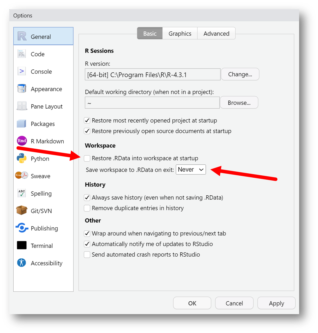
This would be like when you are baking, and you follow the recipe, but then you add in some cinnamon and nutmeg which the recipe doesn’t call for. You also measure out some extra chocolate chips and brown sugar, but you end up not using that. The cookies come out fantastic and you want to make them again. You open up your kitchen and the cinnamon, nutmeg, chocolate chips and brown sugar are all there, but nothing says that you need them in your recipe. We don’t want to keep all the old information. We only want what is in the recipe (after we update it to include the extra spices).
Decorate
Navigate to Tools > Global Options > Appearance
This is all yours! Take ownership and find a cool theme that you like. Make it look nice and how you want it.
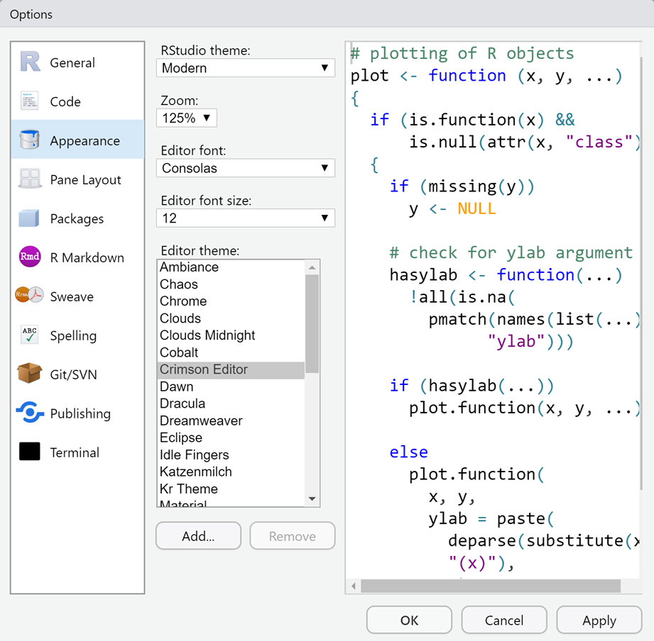
Right now I am rocking the “Chaos” theme with my fonts a little larger because apparently I am getting older.
Intro to Data Wrangling
Special thanks to Sara J. Weston and the work done with their class at Oregon.
This is currently under development and is being adapted from a previous assignment. To view things in it’s entirety, navigate to https://docs.google.com/document/d/188JrtiKyjGGu57rKtEyzPF7EhKeRwqBkB7lqhQw4daQ/edit?usp=sharing
Goal
The focus of this section is to introduce you to some simple tools that will allow you to calculate, visualize and manipulate the data in R. We will use some of the skills we worked through during our class on introducing R, such as creating objects, working with and loading in data, installing packages as well as learning how to use some new functions.
Recap: Directory - Where’s my file??
R Project
We will be going over using the R Project in class, but in case there are still some lingering questions, these resources are extremely helpful.
<https://uopsych.github.io/psy611/labs/lab-1.html#projects> <https://martinctc.github.io/blog/rstudio-projects-and-working-directories-a-beginner%27s-guide/> A directory refers to a file path (location on your computer). A working directory in R is the default file path where R will read and save files. You can check your current working directory by typing getwd() in the console.
getwd() [1] "C:/Users/Dustin_Haraden/Documents"Because I am working on a PC, subfolders are separated by \. Alternatively, if you use a Mac, subfolders will be separated by /.
Since we are going to be using the here() package, this will update the default file path from what you get above to where you have opened your R-Notebook. Basically you are telling R, “Hey! Look right here where I opened this file. I want you to stay right here and not wander off to another part of my computer. If you do, I will be very sad. Please don’t do that to me.”
Whenever starting a new project/analysis, it will be helpful to create a different folder to include all of the information. This folder will also have your R Project file to again, inform A sample of this could be something like this:
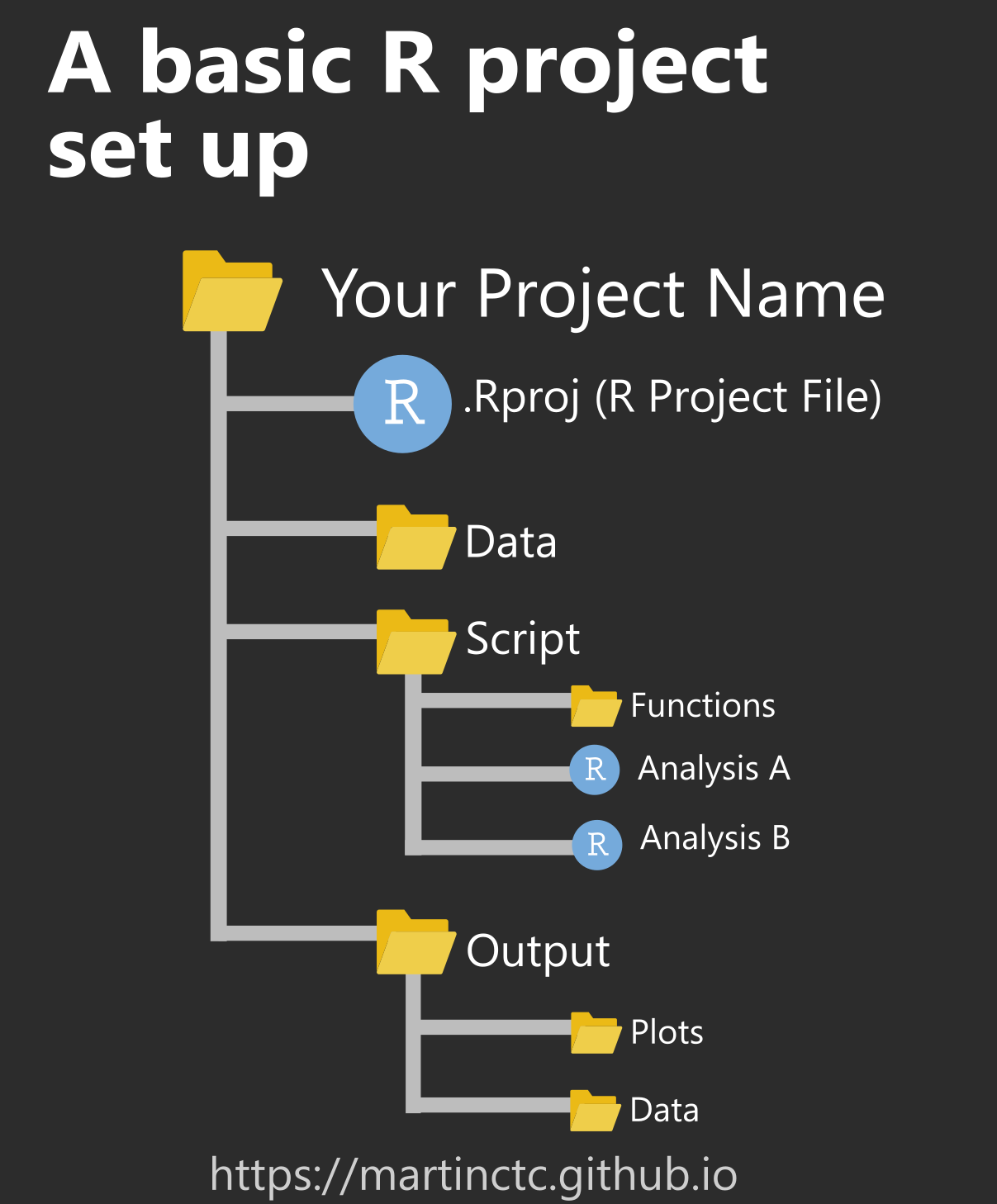
Getting Started
Create a reproducible lab report
To create your new lab report, in RStudio, go to New File -> R Markdown. Then delete everything after Line 5 and save it in the folder you will be using for the current lab. Remember, make a single folder on your computer that holds everything necessary for the project you are working on.
Put the Data where it needs to be
Download your data that you will be using and place this data file in the folder you are using. I always encourage a “Data” Folder that holds all raw data.
Load the Libraries
Get the libraries loaded in their own code chunk. We will be using here, psych and rio. Remember that if you haven’t already installed these libraries (i.e., bought the book from the book store for your own personal library), you will need to run the command install.packages() in the console with the appropriate packages name in the parentheses surrounded by quotation marks.
In the console:
install.packages("here") install.packages("tidyverse") install.packages("rio")In the first code chunk of your Rmd file
library(here) library(tidyverse) library(rio)Import the data
Import the data using the rio package and save it to an object called sleep_data. You will be able to use the import() function as well as the here() function.
| sleep_data <- import(here(“Labs”, “Data”, “SleepFile”, “SleepData.sav”)) |
Visualizing Distributions
Recall from lecture that a distribution often refers to a description of the (relative) number of times a given variable will take each of its unique values.
Histogram
One common way of visualizing distributions is using a histogram, which plots the frequencies of different values for a given variable.
For example, let’s take a look at a distribution of the age variable. We do this using the hist() function. (Remember, you can check out the help documentation using ?hist).
Create a histogram using the age variable with the title “Histogram of Age” and the x-axis labeled as “Age”.
You can also change the number of bins (i.e. bars) in your histogram using the breaks argument. Try 5, 10, and 20 breaks. What do you notice as the number of breaks increases?
Boxplot
Another way to visualize distribution and to better examine the outliers is to use a boxplot. For a short guide on how to read boxplots, seehere or refer tothis section of the textbook.
Create a boxplot using the age variable with the title “Boxplot of Age” and the x-axis labeled as “Age”. What do you notice??
Investigate the distribution more with boxplot.stats(x = sleep_data$age)$out
Looking into the future…
So far we have been plotting in base R. However, theggplot2 package is generally a much better tool for plotting. For now we’ll stick with base plotting to keep things simple, but in a future class you will learn how to use ggplot to make better-looking plots, such as this:
Ok, so now that we know how to visualize a basic distribution, let’s think about how we commonly characterize distributions with descriptive statistics…
Basic Descriptives
Measures of Central Tendency
For a given set of observations, measures of central tendency allow us to get the “gist” of the data. They tell us about where the “average” or the “mid-point” of the data lies. Let’s take a look at the data that we have already loaded in, and complete some of these tasks (which we may already have done in previous classes).
Mean
A quick way to find the mean is to use the aptly named mean() function from base R. Use this function on the age variable in the sleep_data dataset.
| mean(sleep_data$age) |
Oh no! We forgot to account for the missing variables in our variable! We got NA! The reason for this is that the mean is calculated by using every value for a given variable, so if you don’t remove (or impute) the missing values before getting the mean, it won’t work.
Let’s try that again, but using the additional argument to eliminate (or remove) the NA’s from the variable prior to computing the mean.
| mean(sleep_data$age, na.rm = TRUE) |
Median
The median is the middle value of a set of observations: 50% of the data points fall below the median, and 50% fall above.
To find the median, we can use the median() function. Use it on the age variable.
Measures of Variability
Range
The range gives us the distance between the smallest and largest value in a dataset. You can find the range using the range() function, which will output the minimum and maximum values. Find the range of the age variable.
Variance and Standard Deviation
To find the variance and standard deviation, we use var() and sd(), respectively. Find the variance and standard deviation of the age variable.
Summarizing Data
So far we have been calculating various descriptive statistics (somewhat painstakingly) using an assortment of different functions. So what if we have a dataset with a bunch of variables we want descriptive statistics for? Surely we don’t want to calculate descriptives for each variable by hand…
Fortunately for us, there is a function called describe() from the {psych} package, which we can use to quickly summarize a whole set of variables in a dataset.
Be sure to first install the package prior to putting it into your library code chunk. Reminder: anytime you add a library, be sure you actually run the code line library(psych). Otherwise, you will have a hard time trying to use the next functions.
Let’s use it with our sleep dataset!
describe()
This function automatically calculates all of the descriptives we reviewed above (and more!). Use the describe() function from the psych package on the entire sleep_data dataset.
Notes: If you load a library at the beginning, you can directly call any function from it. Instead, you can call a function by library_name::function_name without loading the entire library.
psych::describe(sleep_data) # or if you have already loaded the library describe(sleep_data) |
NOTE: Some variables are not numeric and are categorical variables of type character. By default, the describe() function forces non-numeric variables to be numeric and attempts to calculate descriptives for them. These variables are marked with an asterisk (*). In this case, it doesn’t make sense to calculate descriptive statistics for these variables, so we get a warning message and a bunch of NaN’s and NA’s for these variables.
A better approach would be to remove non-numeric variables before you attempt to run numerical calculations on your dataset.
Now let’s take a closer look at trying to update the age variable in this dataset.
Intro to the tidyverse
The tidyverse, according to its creators, is “an opinionated collection of R packages designed for data science.” It’s a suite of packages designed with a consistent philosophy and aesthetic. This is nice because all of the packages are designed to work well together, providing a consistent framework to do many of the most common tasks in R, including, but not limited to…
data manipulation (dplyr) = our focus today
reshaping data (tidyr)
data visualization (ggplot2)
working with strings (stringr)
working with factors (forcats)
To load all the packages included in the tidyverse, use:
# if you need to install, use install.packages(‘tidyverse’) library(tidyverse) library(dplyr) |
Three qualities of the tidyverse are worth mentioning at the outset:
Packages are designed to be like grammars for their task, so we’ll be using functions that are named as verbs to discuss the tidyverse. The idea is that you can string these grammatical elements together to form more complex statements, just like with language.
The first argument of (basically) every function we’ll review today is data (in the form of a data frame). This is very handy, especially when it comes to piping (discussed below).
Variable names are usually not quoted.
What is data wrangling?
Data wrangling, broadly speaking, means getting your data into a useful form for visualizing and modeling it. Hadley Wickham, who has developed a lot of the tidyverse, conceptualizes the main steps involved in data wrangling as follows:
Importing your data
Tidying your data (see brief overview below)
Transforming your data (what we’ll cover today)
The figure below highlights the steps in data wrangling in relation to the broader scope of a typical data science workflow:
What is “tidy data”?
Data is considered “tidy” when:
Each variable has its own column
Each observation has its own row
Each value has its own cell
The following figure is from R for Data Science and visualizes tidy data.
If your data is not already in tidy format when you import it, you can use functions from the {tidyR} package, e.g. pivot_longer() and pivot_wider(), that allow you to “reshape” your data to get it into tidy format.
However, this term we are mostly going to work with simpler datasets that are already tidy, so we are not going to focus on these functions today. These functions will become especially useful in the future when we work with repeated measures data that has multiple observations for each subject. If you are interested in learning more about reshaping your data with {tidyR}, check out this chapter from R for Data Science.
{dplyr}
Most of the functions we’ll go over today come from the {dplyr} package. Essentially, you can think of this package as a set of “pliers” that you can use to tweak data frames, hence its name (and hex sticker).
{dplyr} is a “grammar” of data manipulation. As such, its functions are verbs:
mutate() adds new variables that are functions of existing variables
select() picks variables based on their names.
filter() picks cases based on their values.
summarize() reduces multiple values down to a single summary.
arrange() changes the ordering of the rows.
Note that {dplyr} functions always take a data frame as the first argument and return a modified data frame back to you. The fact that you always get a data frame back is useful down the road when you are modeling and visualizing data.
Pipes
Pipes come from the {magrittr} package are available when you load the tidyverse. (Technically, the pipe is imported with {dplyr}.) Pipes are a way to write strings of functions more easily, creating pipelines. They are extremely powerful and useful. A pipe looks like this:
You can enter a pipe with the shortcut CTRL+Shift+M for PC or CMD+Shift+M for Mac.
A pipe passes an object on the left-hand side as the first argument (or . argument) of whatever function is on the right-hand side.
x %>% f(y) is the same as f(x, y)
y %>% f(x, ., z) is the same as f(x, y, z )
Example: I want to calculate the mean of the mpg variable from the mtcars data set and round our answer to 2 decimal places. I can accomplish this by nesting:
| round(mean(mtcars$mpg, na.rm = TRUE), 2) |
Or, we could use pipes. Grammatically, you can think of a pipe as “then.” I have a variable, the mile per gallon of cars, THEN I want to take the mean of that variable, and THEN I want to round that answer to two decimal places.
mtcars$mpg %>% # select the `mpg` variable from the `mtcars` dataset mean(na.rm = TRUE) %>% # calculate the mean round(2) # round to 2 decimal places |
Now try rewriting the following code using pipes:
| round(sqrt(sum(mtcars$cyl)), 1) |
Why use pipes?
Cleaner code
- This is nice, because it helps make your code more readable by other humans (including your future self).
Cleaner environment
When you use pipes, you have basically no reason to save objects from intermediary steps in your data wrangling / analysis workflow, because you can just pass output from function to function without saving it.
Finding objects you’re looking for is easier.
Efficiency in writing code
- Naming objects is hard; piping means coming up with fewer names.
More error-proof
- Because naming is hard, you might accidentally re-use a name and make an error.
Manipulating Observations
Extract rows with filter()
The filter() function is used to subset observations based on their values. The result of filtering is a data frame with the same number of columns as before but fewer rows, as illustrated below…
The first argument is data and subsequent arguments are logical expressions that tell you which observations to retain in the data frame.
For example, we can filter rows to retain data only for the students who do not have a roommate.
sleep_data %>% filter(roommate == 2) |
But we may want to save this as a new datafile. Can assign this to a new object.
Logical Operators
The == we just used is an example of a comparison operator that tests for equality. The other comparison operators available are :
> (greater than)
>= (greater than or equal to)
< (less than)
<= (less than or equal to)
!= (not equal to)
You can combine multiple arguments to filter() with Boolean operators. The figure below fromR for Data Science shows the complete set of Boolean operators.
Try it out yourself:
First, let’s filter for observations that are greater than the mean of age
sleep_data %>% filter(age > mean(age, na.rm = TRUE) |
Now, you try filtering observations that are greater than the mean of happiness, but the participant does have a roommate:
| # Put your code here |
Filter out the age variable that are out of bounds
Manipulating Variables
Extract columns with select()
The select() function subsets columns in your data frame. This is particularly useful when you have a data set with a huge number of variables and you want to narrow down to the variables that are relevant for your analysis.
The first argument is data, followed by the name(s) of the column(s) you want to subset. Note that you can use variable positions rather than their names, but this is usually not as useful. Let’s go through some simple examples of common uses of select().
Select one variable
sleep_data %>% select(bed_study) |
Select multiple variables
sleep_data %>% select(bed_study, bed_read, bed_friends) |
Select a range of variables
sleep_data %>% select(bed_study:bed_videogames) %>% names() |
De-select variables with a minus sign (-)
sleep_data %>% select(-age) |
De-select range of variables
Note: everything() is a helper function that gives us all the remaining variables in the data frame (see more onhelper functions below)
sleep_data %>% select(-(ESS1:everything()) |
Helper functions for select()
There are some “helper” functions that you can use along with select() that can sometimes be more efficient than selecting your variables explicitly by name.
| function | what it does |
| starts_with() | selects columns starting with a string |
| ends_with() | selects columns that end with a string |
| contains() | selects columns that contain a string |
| matches() | selects columns that match a regular expression |
| num_ranges() | selects columns that match a numerical range |
| one_of() | selects columns whose names match entries in a character vector |
| everything() | selects all columns |
| last_col() | selects last column; can include an offset. |
Quick example:
sleep_data %>% select(starts_with(“a”) |
Make new variables with mutate()
The mutate() function is most commonly used to add new columns to your data frame that are functions of existing columns.
mutate() requires data as its first argument, followed by a set of expressions defining new columns. Let’s take a couple examples…
Create new variables
- Note: New variables are automatically added at the end of the data frame (scroll to the right to see them)
sleep_data <- sleep_data %>% mutate(ess_sum = ESS1 + ESS2 + ESS3 + ESS4 + ESS5 + ESS6 + ESS7 + ESS8) |