Tables & Reporting

Using the Power of R-Markdown

We are going to explore some of the useful libraries to report tables in R, and try to capitalize on how R knits information. The goal is to have all analyses and the text in a single document that will update as necessary.

There won’t be any slides with this one, we will just work on doing some coding together!

Let’s start with a new file and adding in a new dataset. It is good to continuously check to make sure that your code is reproducible by closing your project often or restarting R.

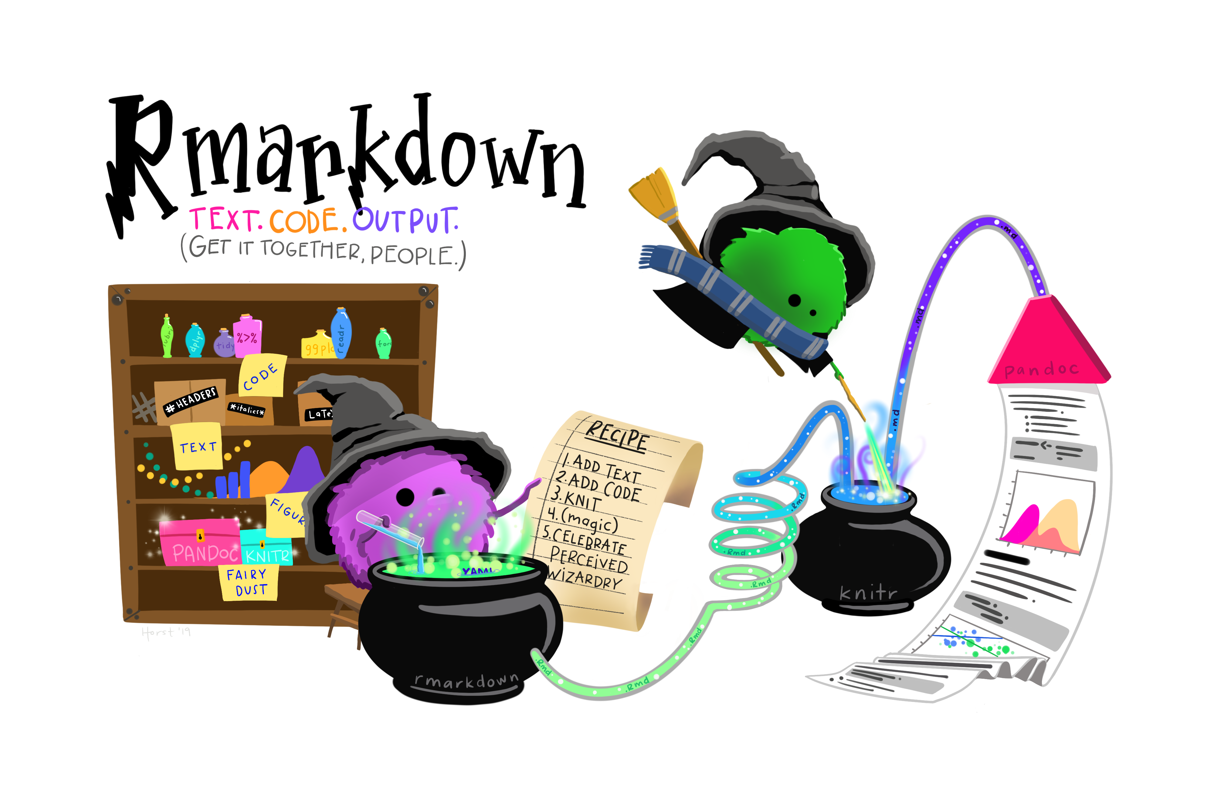
Dark R’s Dark Rs (.Rmd)

When starting a file, I like to have all libraries and setup in the initial block. This makes sure that everything is covered and whenever I share this file, those receiving it will be aware of how to get started.

library(here) #relative file path

here() starts at /home/runner/work/aware-stats_2025/aware-stats_2025

library(rio) #import data
library(easystats) #collection of tools

# Attaching packages: easystats 0.7.5 (red = needs update)
✔ bayestestR  0.17.0   ✔ correlation 0.8.8 
✔ datawizard  1.2.0    ✔ effectsize  1.0.1 
✔ insight     1.4.2    ✔ modelbased  0.13.0
✔ performance 0.15.1   ✖ parameters  0.28.1
✔ report      0.6.1    ✔ see         0.11.0

Restart the R-Session and update packages with `easystats::easystats_update()`.

library(dplyr) #data wrangling

Attaching package: 'dplyr'

The following objects are masked from 'package:stats':

    filter, lag

The following objects are masked from 'package:base':

    intersect, setdiff, setequal, union

library(ggplot2) #data visualization
library(psych) #cronbach alpha (and a whole lot of other stuff)

Attaching package: 'psych'

The following objects are masked from 'package:ggplot2':

    %+%, alpha

The following object is masked from 'package:effectsize':

    phi

The following object is masked from 'package:datawizard':

    rescale

library(janitor) #cleaning variable names

Attaching package: 'janitor'

The following object is masked from 'package:insight':

    clean_names

The following objects are masked from 'package:datawizard':

    remove_empty, remove_empty_rows

The following objects are masked from 'package:stats':

    chisq.test, fisher.test

library(sjPlot) #making nice tables
library(broom)

#tell R not to display scientific notation
options(scipen=999)

# Create a list of citations of the libraries that are used
report::cite_packages()

  - Ben-Shachar MS, Lüdecke D, Makowski D (2020). "effectsize: Estimation of Effect Size Indices and Standardized Parameters." _Journal of Open Source Software_, *5*(56), 2815. doi:10.21105/joss.02815 <https://doi.org/10.21105/joss.02815>, <https://doi.org/10.21105/joss.02815>.
  - Chan C, Leeper T, Becker J, Schoch D (2023). _rio: A Swiss-army knife for data file I/O_. <https://cran.r-project.org/package=rio>.
  - Firke S (2024). _janitor: Simple Tools for Examining and Cleaning Dirty Data_. R package version 2.2.1, <https://github.com/sfirke/janitor>.
  - Lüdecke D (2025). _sjPlot: Data Visualization for Statistics in Social Science_. R package version 2.9.0, <https://CRAN.R-project.org/package=sjPlot>.
  - Lüdecke D, Ben-Shachar M, Patil I, Makowski D (2020). "Extracting, Computing and Exploring the Parameters of Statistical Models using R." _Journal of Open Source Software_, *5*(53), 2445. doi:10.21105/joss.02445 <https://doi.org/10.21105/joss.02445>.
  - Lüdecke D, Ben-Shachar M, Patil I, Waggoner P, Makowski D (2021). "performance: An R Package for Assessment, Comparison and Testing of Statistical Models." _Journal of Open Source Software_, *6*(60), 3139. doi:10.21105/joss.03139 <https://doi.org/10.21105/joss.03139>.
  - Lüdecke D, Ben-Shachar M, Patil I, Wiernik B, Bacher E, Thériault R, Makowski D (2022). "easystats: Framework for Easy Statistical Modeling, Visualization, and Reporting." _CRAN_. doi:10.32614/CRAN.package.easystats <https://doi.org/10.32614/CRAN.package.easystats>, R package, <https://easystats.github.io/easystats/>.
  - Lüdecke D, Patil I, Ben-Shachar M, Wiernik B, Waggoner P, Makowski D (2021). "see: An R Package for Visualizing Statistical Models." _Journal of Open Source Software_, *6*(64), 3393. doi:10.21105/joss.03393 <https://doi.org/10.21105/joss.03393>.
  - Lüdecke D, Waggoner P, Makowski D (2019). "insight: A Unified Interface to Access Information from Model Objects in R." _Journal of Open Source Software_, *4*(38), 1412. doi:10.21105/joss.01412 <https://doi.org/10.21105/joss.01412>.
  - Makowski D, Ben-Shachar M, Lüdecke D (2019). "bayestestR: Describing Effects and their Uncertainty, Existence and Significance within the Bayesian Framework." _Journal of Open Source Software_, *4*(40), 1541. doi:10.21105/joss.01541 <https://doi.org/10.21105/joss.01541>, <https://joss.theoj.org/papers/10.21105/joss.01541>.
  - Makowski D, Ben-Shachar M, Wiernik B, Patil I, Thériault R, Lüdecke D (2025). "modelbased: An R package to make the most out of your statistical models through marginal means, marginal effects, and model predictions." _Journal of Open Source Software_, *10*(109), 7969. doi:10.21105/joss.07969 <https://doi.org/10.21105/joss.07969>, <https://joss.theoj.org/papers/10.21105/joss.07969>.
  - Makowski D, Lüdecke D, Patil I, Thériault R, Ben-Shachar M, Wiernik B (2023). "Automated Results Reporting as a Practical Tool to Improve Reproducibility and Methodological Best Practices Adoption." _CRAN_. <https://easystats.github.io/report/>.
  - Makowski D, Wiernik B, Patil I, Lüdecke D, Ben-Shachar M (2022). "correlation: Methods for Correlation Analysis." Version 0.8.3, <https://CRAN.R-project.org/package=correlation>. Makowski D, Ben-Shachar M, Patil I, Lüdecke D (2020). "Methods and Algorithms for Correlation Analysis in R." _Journal of Open Source Software_, *5*(51), 2306. doi:10.21105/joss.02306 <https://doi.org/10.21105/joss.02306>, <https://joss.theoj.org/papers/10.21105/joss.02306>.
  - Müller K (2020). _here: A Simpler Way to Find Your Files_. R package version 1.0.1, <https://here.r-lib.org/>.
  - Patil I, Makowski D, Ben-Shachar M, Wiernik B, Bacher E, Lüdecke D (2022). "datawizard: An R Package for Easy Data Preparation and Statistical Transformations." _Journal of Open Source Software_, *7*(78), 4684. doi:10.21105/joss.04684 <https://doi.org/10.21105/joss.04684>.
  - R Core Team (2025). _R: A Language and Environment for Statistical Computing_. R Foundation for Statistical Computing, Vienna, Austria. <https://www.R-project.org/>.
  - Robinson D, Hayes A, Couch S (2025). _broom: Convert Statistical Objects into Tidy Tibbles_. R package version 1.0.9, <https://broom.tidymodels.org/>.
  - Wickham H (2016). _ggplot2: Elegant Graphics for Data Analysis_. Springer-Verlag New York. ISBN 978-3-319-24277-4, <https://ggplot2.tidyverse.org>.
  - Wickham H, François R, Henry L, Müller K, Vaughan D (2023). _dplyr: A Grammar of Data Manipulation_. R package version 1.1.4, <https://dplyr.tidyverse.org>.
  - William Revelle (2025). _psych: Procedures for Psychological, Psychometric, and Personality Research_. Northwestern University, Evanston, Illinois. R package version 2.5.6, <https://CRAN.R-project.org/package=psych>.

# Identify the version of R and the type of machine that is running it
report::report_system()

Analyses were conducted using the R Statistical language (version 4.5.1; R Core
Team, 2025) on Ubuntu 24.04.3 LTS

# Create a list of the package names and the in-text citation 
#report::report_packages()

# Import the data

cah <- import(here("files", "data", "CAH_Data.csv")) %>% 
  clean_names()

tipi <- import(here("files", "data", "final_tipi.csv"))

These data are coming from a dataset curated by Cards Against Humanity and their “Pulse of the Nation” survey. You can find more data here.

Tables - sjPlot

Sometimes there will be a data visualization that is needed or even some tables of descriptives. When generating tables, I tend to prefer to use sjPlot (https://strengejacke.github.io/sjPlot/index.html)

cah %>% 
  describe() %>% 
  tibble::rownames_to_column() %>% 
  select(c(rowname, n, mean, sd)) %>% 
  tab_df(title = "Table 1 - Descriptive Statistics")

Table 1 - Descriptive Statistics

rowname	n	mean	sd
id	1000	500.50	288.82
income	456	89589.91	72275.00
gender*	1000	2.54	0.56
age	1000	49.41	16.63
age_range*	1000	3.91	1.55
political_affiliation*	1000	2.63	0.97
education*	1000	3.71	1.60
ethnicity*	1000	5.04	1.55
marrital_status*	1000	4.71	1.79
climate_change*	1000	2.91	0.77
transformers	938	1.33	1.56
books	977	22.33	75.87
ghosts*	1000	2.35	0.53
spending*	1000	2.84	1.12
choice*	1000	2.32	0.65
shower_pee*	1000	2.40	0.67

cah %>% 
  select(c(age, income, books, transformers)) %>% 
  tab_corr(title = "Table 2 - Correlations", 
           triangle = "lower", 
           var.labels = c("Age", "Income", "# of books", "# of Transformers Movies"))

Table 2 - Correlations

	Age	Income	# of books	# of Transformers Movies
Age
Income	-0.068
# of books	0.009	-0.058
# of Transformers Movies	-0.212***	-0.094	0.093
Computed correlation used pearson-method with listwise-deletion.

Statistical Models

Then the next section will be broken up into my research questions and will have the corresponding modeling. Below are some examples of what that could look like.

We will also explore the

Linear Regression

model1 <- lm(income ~ gender + ghosts + transformers, 
             data = cah)

summary(model1)

Call:
lm(formula = income ~ gender + ghosts + transformers, data = cah)

Residuals:
    Min      1Q  Median      3Q     Max 
-109052  -47436  -10890   30110  418110 

Coefficients:
             Estimate Std. Error t value       Pr(>|t|)    
(Intercept)    131052      20263   6.468 0.000000000271 ***
genderMale      22499       7362   3.056        0.00238 ** 
genderOther      5164      19889   0.260        0.79525    
ghostsNo       -49162      20468  -2.402        0.01673 *  
ghostsYes      -42491      20795  -2.043        0.04163 *  
transformers    -4485       2257  -1.987        0.04756 *  
---
Signif. codes:  0 '***' 0.001 '**' 0.01 '*' 0.05 '.' 0.1 ' ' 1

Residual standard error: 71820 on 431 degrees of freedom
  (563 observations deleted due to missingness)
Multiple R-squared:  0.04017,   Adjusted R-squared:  0.02904 
F-statistic: 3.608 on 5 and 431 DF,  p-value: 0.003301

tab_model(model1, 
          title = "Table 3 - Predicting Income", 
          dv.labels = "Income")

Table 3 - Predicting Income

	Income
Predictors	Estimates	CI	p
(Intercept)	131052.10	91225.38 – 170878.83	<0.001
gender [Male]	22498.61	8027.80 – 36969.41	0.002
gender [Other]	5164.40	-33927.86 – 44256.66	0.795
ghosts [No]	-49161.65	-89390.62 – -8932.69	0.017
ghosts [Yes]	-42490.66	-83362.88 – -1618.43	0.042
transformers	-4484.98	-8921.49 – -48.47	0.048
Observations	437
R2 / R2 adjusted	0.040 / 0.029

report(model1)

We fitted a linear model (estimated using OLS) to predict income with gender,
ghosts and transformers (formula: income ~ gender + ghosts + transformers). The
model explains a statistically significant and weak proportion of variance (R2
= 0.04, F(5, 431) = 3.61, p = 0.003, adj. R2 = 0.03). The model's intercept,
corresponding to gender = Female, ghosts = and transformers = 0, is at 1.31e+05
(95% CI [91225.38, 1.71e+05], t(431) = 6.47, p < .001). Within this model:

  - The effect of gender [Male] is statistically significant and positive (beta =
22498.61, 95% CI [8027.80, 36969.41], t(431) = 3.06, p = 0.002; Std. beta =
0.31, 95% CI [0.11, 0.51])
  - The effect of gender [Other] is statistically non-significant and positive
(beta = 5164.40, 95% CI [-33927.86, 44256.66], t(431) = 0.26, p = 0.795; Std.
beta = 0.07, 95% CI [-0.47, 0.61])
  - The effect of ghosts [No] is statistically significant and negative (beta =
-49161.65, 95% CI [-89390.62, -8932.69], t(431) = -2.40, p = 0.017; Std. beta =
-0.67, 95% CI [-1.23, -0.12])
  - The effect of ghosts [Yes] is statistically significant and negative (beta =
-42490.66, 95% CI [-83362.88, -1618.43], t(431) = -2.04, p = 0.042; Std. beta =
-0.58, 95% CI [-1.14, -0.02])
  - The effect of transformers is statistically significant and negative (beta =
-4484.98, 95% CI [-8921.49, -48.47], t(431) = -1.99, p = 0.048; Std. beta =
-0.10, 95% CI [-0.19, -1.03e-03])

Standardized parameters were obtained by fitting the model on a standardized
version of the dataset. 95% Confidence Intervals (CIs) and p-values were
computed using a Wald t-distribution approximation.

model1$coefficients[6]

transformers 
   -4484.981 

transformers_beta <- broom::tidy(model1) %>% 
  filter(term == "transformers") %>% 
  select(estimate)

Sample 1 We ran a linear regression model to predict income and found that the number of transformers movies significantly predicted a lower income (b = -4484.98)

Sample 2 - Broom We ran a linear regression model to predict income and found that the number of transformers movies significantly predicted a lower income (b = -4484.981256)

Some example code chunks

Cool library to work with missing data! install.packages('misty') https://www.rdocumentation.org/packages/misty/versions/0.7.1

Reverse Scoring

#https://easystats.github.io/datawizard/reference/reverse.html

## Reverse Scoring

#cleanr <- reverse(data, 
#                  select = c(BFI_6_T1, BFI_21_T1, BFI_31_T1))

Easily identify Duplicates

#https://easystats.github.io/datawizard/reference/data_duplicated.html

## Identify Duplicates

#duplicate_raw <- data_duplicated(raw, select = "id")

Generate Cronbach’s Alpha

## Cronbach's Alpha
#dat %>% 
#  select(BPAQ_1, BPAQ_2, BPAQ_3, BPAQ_4, BPAQ_5) %>% 
#  psych::alpha()

More fun stuff we can explore:

🔗rticles - https://pkgs.rstudio.com/rticles/

• This will provide templates for various journal articles

🔗papaja - https://github.com/crsh/papaja?tab=readme-ov-file

• Another library that generates APA style articles (Preparing APA Journal Articles)

• Also aids in the formatting of the reporting in text